# Install and load libraries.
library(xlsx)
## Loading required package: rJava
## Loading required package: xlsxjars
library(plyr)
# Import data from 'homework5data.xlsx' using xlsx function.
pain.data <- read.xlsx("pain.xlsx", sheetName = "pain", header = TRUE)
head(pain.data) ; tail(pain.data)
##       Treatment Age Severe Pain
## 1 New Treatment  29      1    1
## 2 New Treatment  39      0    0
## 3 New Treatment  43      0    0
## 4 New Treatment  27      0    1
## 5 New Treatment  16      1    1
## 6 New Treatment  39      0    0
##     Treatment Age Severe Pain
## 195   Placebo  57      0    0
## 196   Placebo  66      1    0
## 197   Placebo  56      0    0
## 198   Placebo  50      0    0
## 199   Placebo  39      0    1
## 200   Placebo  49      0    0
# View summary of pain.data
summary(pain.data)
##          Treatment        Age            Severe           Pain
##  New Treatment:100   Min.   :10.00   Min.   :0.000   Min.   :0.00
##  Placebo      :100   1st Qu.:38.75   1st Qu.:0.000   1st Qu.:0.00
##                      Median :48.00   Median :0.000   Median :0.00
##                      Mean   :47.60   Mean   :0.275   Mean   :0.26
##                      3rd Qu.:56.00   3rd Qu.:1.000   3rd Qu.:1.00
##                      Max.   :81.00   Max.   :1.000   Max.   :1.00
str(pain.data)
## 'data.frame':    200 obs. of  4 variables:
##  $ Treatment: Factor w/ 2 levels "New Treatment",..: 1 1 1 1 1 1 1 1 1 1 ...
##  $ Age      : num  29 39 43 27 16 39 51 35 39 52 ...
##  $ Severe   : num  1 0 0 0 1 0 1 0 1 0 ...
##  $ Pain     : num  1 0 0 1 1 0 0 0 0 0 ...
#-------------
# Question 1.
#-------------
# Summarize data relating to pain by treatment type.
ddply(pain.data, "Treatment", summarise,
      N = length(Pain),
      Mild_to_No = length(Pain[Pain == 0]),
      Mod_to_Sev = length(Pain[Pain == 1]),
      P_Mild_to_No = Mild_to_No / N,
      P_Mod_to_Sev = Mod_to_Sev / N)
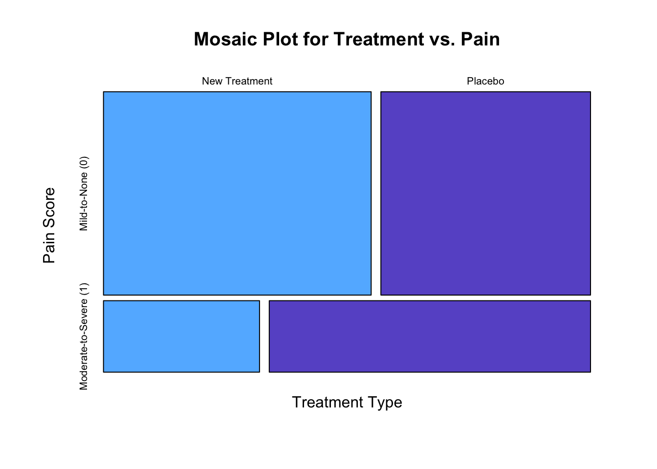
##       Treatment   N Mild_to_No Mod_to_Sev P_Mild_to_No P_Mod_to_Sev
## 1 New Treatment 100         83         17         0.83         0.17
## 2       Placebo 100         65         35         0.65         0.35
# Generate a mosaic plot for pain score by treatment type.
x <- matrix(table(pain.data$Treatment, pain.data$Pain), ncol = 2, byrow = TRUE)
colnames(x) <- c("New Treatment", "Placebo")
rownames(x) <- c("Mild-to-None (0)", "Moderate-to-Severe (1)")
mosaicplot(x, dir = c("h", "v"),
           main = "Mosaic Plot for Treatment vs. Pain",
           xlab = "Treatment Type", ylab = "Pain Score", type = "n",
           col = c("steelblue1", "slateblue3"))
#-------------
# Question 2.
#-------------
# Determine test statistic to compare against.
qnorm(0.975)
## [1] 1.959964
# Test moderate-to-severe pain between treatment groups.
prop.test(c(17, 35), c(100, 100), alternative = "two.sided",
          conf.level = 0.95, correct = FALSE)
##
##  2-sample test for equality of proportions without continuity
##  correction
##
## data:  c(17, 35) out of c(100, 100)
## X-squared = 8.42, df = 1, p-value = 0.003711
## alternative hypothesis: two.sided
## 95 percent confidence interval:
##  -0.29899419 -0.06100581
## sample estimates:
## prop 1 prop 2
##   0.17   0.35
#-------------
# Question 3.
#-------------
# Perform logistic regression with treatment as only explantory variable.
# Control new treatment variable for regression.
pain.data$Treatment_New <- ifelse(pain.data$Treatment == "New Treatment", 1, 0)
m1 <- glm(pain.data$Pain ~ pain.data$Treatment_New, family = binomial)
summary(m1)
##
## Call:
## glm(formula = pain.data$Pain ~ pain.data$Treatment_New, family = binomial)
##
## Deviance Residuals:
##     Min       1Q   Median       3Q      Max
## -0.9282  -0.9282  -0.6105   1.4490   1.8825
##
## Coefficients:
##                         Estimate Std. Error z value Pr(>|z|)
## (Intercept)              -0.6190     0.2097  -2.953  0.00315 **
## pain.data$Treatment_New  -0.9666     0.3389  -2.852  0.00434 **
## ---
## Signif. codes:  0 '***' 0.001 '**' 0.01 '*' 0.05 '.' 0.1 ' ' 1
##
## (Dispersion parameter for binomial family taken to be 1)
##
##     Null deviance: 229.22  on 199  degrees of freedom
## Residual deviance: 220.67  on 198  degrees of freedom
## AIC: 224.67
##
## Number of Fisher Scoring iterations: 4
# Control placebo treatement variable for regression.
pain.data$Treatment_Placebo <- ifelse(pain.data$Treatment == "Placebo", 1, 0)
m2 <- glm(pain.data$Pain ~ pain.data$Treatment_Placebo, family = binomial)
summary(m2)
##
## Call:
## glm(formula = pain.data$Pain ~ pain.data$Treatment_Placebo, family = binomial)
##
## Deviance Residuals:
##     Min       1Q   Median       3Q      Max
## -0.9282  -0.9282  -0.6105   1.4490   1.8825
##
## Coefficients:
##                             Estimate Std. Error z value Pr(>|z|)
## (Intercept)                  -1.5856     0.2662  -5.956 2.58e-09 ***
## pain.data$Treatment_Placebo   0.9666     0.3389   2.852  0.00434 **
## ---
## Signif. codes:  0 '***' 0.001 '**' 0.01 '*' 0.05 '.' 0.1 ' ' 1
##
## (Dispersion parameter for binomial family taken to be 1)
##
##     Null deviance: 229.22  on 199  degrees of freedom
## Residual deviance: 220.67  on 198  degrees of freedom
## AIC: 224.67
##
## Number of Fisher Scoring iterations: 4
# Calculate odds ratio for beta coefficient (new treatment).
exp(-0.9666)
## [1] 0.3803741
# Calculate odds ratio for beta coefficient (placebo treatment).
exp(0.9666)
## [1] 2.628991
# Determine 95% confidence intervals for treatments.
exp(cbind(OR = coef(m1), confint.default(m1)))
##                                OR     2.5 %    97.5 %
## (Intercept)             0.5384615 0.3570215 0.8121103
## pain.data$Treatment_New 0.3803787 0.1957834 0.7390203
exp(cbind(OR = coef(m2), confint.default(m2)))
##                                    OR     2.5 %    97.5 %
## (Intercept)                 0.2048193 0.1215531 0.3451243
## pain.data$Treatment_Placebo 2.6289593 1.3531428 5.1076849
# Calculate c-statistic using roc function.
#install.packages("pROC", dependencies = TRUE)
library(pROC)
## Warning: package 'pROC' was built under R version 3.4.4
## Type 'citation("pROC")' for a citation.
##
## Attaching package: 'pROC'
## The following objects are masked from 'package:stats':
##
##     cov, smooth, var
pain.data$prob1 <- predict(m1, type = c("response"))
pain.data$prob1
##   [1] 0.17 0.17 0.17 0.17 0.17 0.17 0.17 0.17 0.17 0.17 0.17 0.17 0.17 0.17
##  [15] 0.17 0.17 0.17 0.17 0.17 0.17 0.17 0.17 0.17 0.17 0.17 0.17 0.17 0.17
##  [29] 0.17 0.17 0.17 0.17 0.17 0.17 0.17 0.17 0.17 0.17 0.17 0.17 0.17 0.17
##  [43] 0.17 0.17 0.17 0.17 0.17 0.17 0.17 0.17 0.17 0.17 0.17 0.17 0.17 0.17
##  [57] 0.17 0.17 0.17 0.17 0.17 0.17 0.17 0.17 0.17 0.17 0.17 0.17 0.17 0.17
##  [71] 0.17 0.17 0.17 0.17 0.17 0.17 0.17 0.17 0.17 0.17 0.17 0.17 0.17 0.17
##  [85] 0.17 0.17 0.17 0.17 0.17 0.17 0.17 0.17 0.17 0.17 0.17 0.17 0.17 0.17
##  [99] 0.17 0.17 0.35 0.35 0.35 0.35 0.35 0.35 0.35 0.35 0.35 0.35 0.35 0.35
## [113] 0.35 0.35 0.35 0.35 0.35 0.35 0.35 0.35 0.35 0.35 0.35 0.35 0.35 0.35
## [127] 0.35 0.35 0.35 0.35 0.35 0.35 0.35 0.35 0.35 0.35 0.35 0.35 0.35 0.35
## [141] 0.35 0.35 0.35 0.35 0.35 0.35 0.35 0.35 0.35 0.35 0.35 0.35 0.35 0.35
## [155] 0.35 0.35 0.35 0.35 0.35 0.35 0.35 0.35 0.35 0.35 0.35 0.35 0.35 0.35
## [169] 0.35 0.35 0.35 0.35 0.35 0.35 0.35 0.35 0.35 0.35 0.35 0.35 0.35 0.35
## [183] 0.35 0.35 0.35 0.35 0.35 0.35 0.35 0.35 0.35 0.35 0.35 0.35 0.35 0.35
## [197] 0.35 0.35 0.35 0.35
roc(pain.data$Pain ~ pain.data$prob1)
##
## Call:
## roc.formula(formula = pain.data$Pain ~ pain.data$prob1)
##
## Data: pain.data$prob1 in 148 controls (pain.data$Pain 0) < 52 cases (pain.data$Pain 1).
## Area under the curve: 0.6169
#-------------
# Question 4.
#-------------
# Perform multiple logistic regression to predict pain from treatment, age, severity.
attach(pain.data)
n1 <- glm(Pain ~ Treatment + Age + Severe, family = "binomial") ; n1
##
## Call:  glm(formula = Pain ~ Treatment + Age + Severe, family = "binomial")
##
## Coefficients:
##      (Intercept)  TreatmentPlacebo               Age            Severe
##           5.5703            2.7612           -0.1933            1.0561
##
## Degrees of Freedom: 199 Total (i.e. Null);  196 Residual
## Null Deviance:       229.2
## Residual Deviance: 136.5     AIC: 144.5
# Perform multiple logistic regression to predict pain using treatment dummy, age, severity.
n2 <- glm(Pain ~ Treatment_New + Age + Severe, family = "binomial") ; n2
##
## Call:  glm(formula = Pain ~ Treatment_New + Age + Severe, family = "binomial")
##
## Coefficients:
##   (Intercept)  Treatment_New            Age         Severe
##        8.3315        -2.7612        -0.1933         1.0561
##
## Degrees of Freedom: 199 Total (i.e. Null);  196 Residual
## Null Deviance:       229.2
## Residual Deviance: 136.5     AIC: 144.5
# Calculate odds ratios given the beta coefficients from regression equation.
exp(n1$coefficients[[2]])
## [1] 15.81889
exp(n1$coefficients[[3]])
## [1] 0.8242507
exp(n1$coefficients[[4]])
## [1] 2.875093
# Calculate odds ratio for age for a 10-yr increase.
exp(n1$coefficients[[3]])
## [1] 0.8242507
exp(n1$coefficients[[3]]*10)
## [1] 0.1447416
# Calculate odds ratios given the beta coefficients from regression equation (with Treatment_New).
exp(n2$coefficients[[2]])
## [1] 0.06321554
exp(n2$coefficients[[3]])
## [1] 0.8242507
exp(n2$coefficients[[4]])
## [1] 2.875093
# Calculate odds ratio for age for a 10-yr increase (with Treatment_ New).
exp(n2$coefficients[[3]])
## [1] 0.8242507
exp(n2$coefficients[[3]]*10)
## [1] 0.1447416
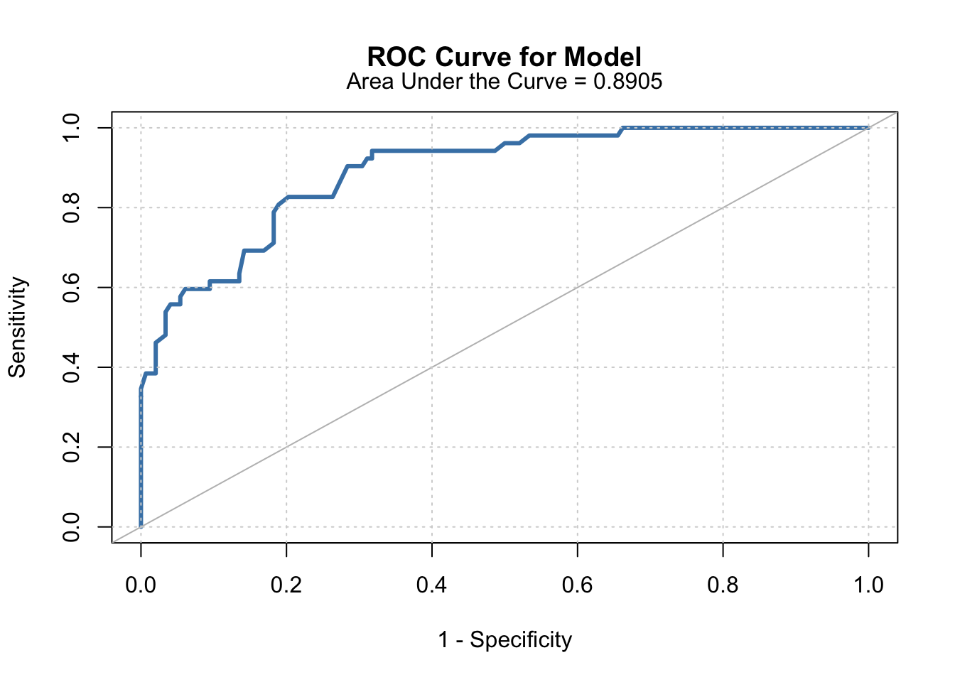
# Calculate c-statistic using roc function.
pain.data$prob2 <- predict(n1, type = c("response"))
roc(pain.data$Pain ~ pain.data$prob2)
##
## Call:
## roc.formula(formula = pain.data$Pain ~ pain.data$prob2)
##
## Data: pain.data$prob2 in 148 controls (pain.data$Pain 0) < 52 cases (pain.data$Pain 1).
## Area under the curve: 0.8905
# Display roc curve.
g <- roc(pain.data$Pain ~ pain.data$prob2)
plot(1-g$specificities, g$sensitivities, type = "l",
     xlab = "1 - Specificity", ylab = "Sensitivity",
     main = "ROC Curve for Model",
     col = "steelblue", lwd = 3)
abline(a = 0, b = 1, col = "gray")
mtext("Area Under the Curve = 0.8905", side = 3, line = 0.65)
grid()
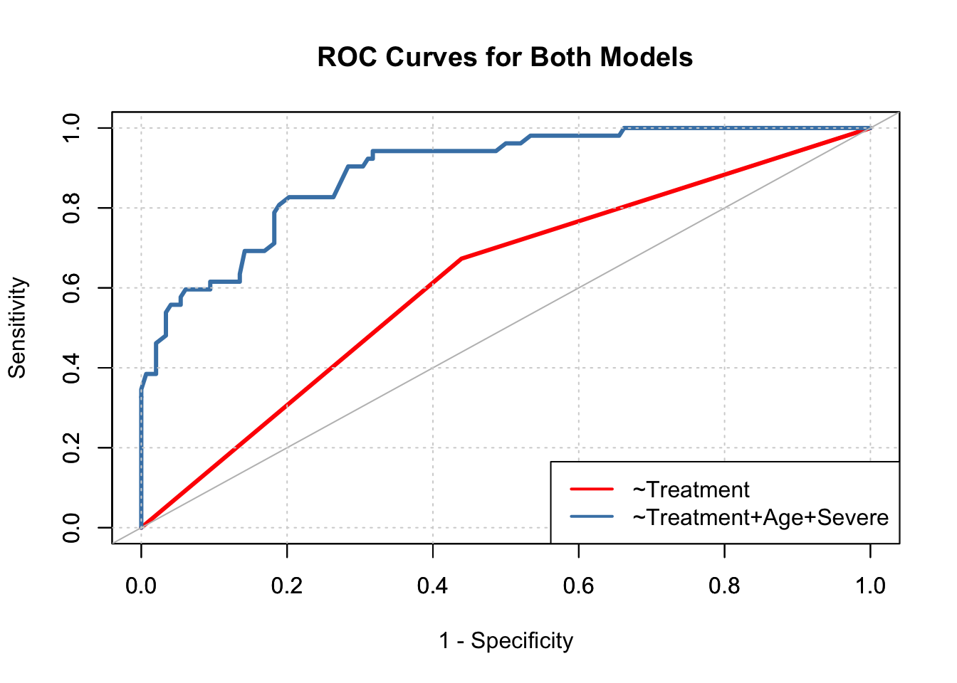
# Display two ROC curves together.
g1 <- roc(pain.data$Pain ~ pain.data$prob1)
g2 <- roc(pain.data$Pain ~ pain.data$prob2)
plot(1-g1$specificities, g1$sensitivities, type = "l",
     xlab = "1 - Specificity", ylab = "Sensitivity",
     main = "ROC Curves for Both Models",
     col = "red", lwd = 3)
par(new = TRUE)
plot(1-g2$specificities, g2$sensitivities, type = "l",
     xlab = "", ylab = "",
     col = "steelblue", lwd = 3)
abline(a = 0, b = 1, col = "gray")
grid()
legend(x = "bottomright", c("~Treatment", "~Treatment+Age+Severe"),
       col = c("red", "steelblue"), lwd = c(2, 2))
# Optional: Look at correlations between variables.
cov2cor(vcov(m1))
##                         (Intercept) pain.data$Treatment_New
## (Intercept)               1.0000000              -0.6187081
## pain.data$Treatment_New  -0.6187081               1.0000000
cov2cor(vcov(n2))
##               (Intercept) Treatment_New        Age     Severe
## (Intercept)     1.0000000    -0.6991441 -0.9784557  0.2274324
## Treatment_New  -0.6991441     1.0000000  0.6275680 -0.2919393
## Age            -0.9784557     0.6275680  1.0000000 -0.3100057
## Severe          0.2274324    -0.2919393 -0.3100057  1.0000000