# Install and load libraries.
library(xlsx)
## Loading required package: rJava
## Loading required package: xlsxjars
# Question 1
# Save the data to Excel and import into R.
data <- read.xlsx("homework3data.xlsx", sheetName = "Sheet1") ; data
##    height selfesteem
## 1      68        4.1
## 2      71        4.6
## 3      62        3.8
## 4      75        4.4
## 5      58        3.2
## 6      60        3.1
## 7      67        3.8
## 8      68        4.1
## 9      71        4.3
## 10     69        3.7
## 11     68        3.5
## 12     67        3.2
## 13     63        3.7
## 14     62        3.3
## 15     60        3.4
## 16     63        4.0
## 17     65        4.1
## 18     67        3.8
## 19     63        3.4
## 20     61        3.6
## 21     58        3.6
## 22     70        4.3
## 23     67        3.3
## 24     65        3.5
## 25     64        4.2
# Question 2
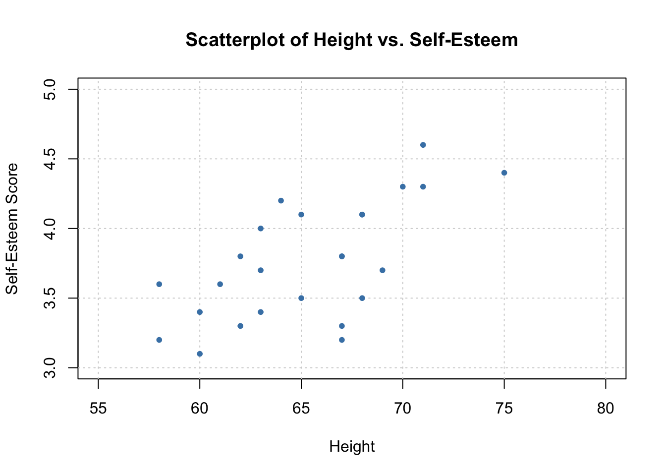
# Generate a scatterplot of the data.
plot(data$height, data$selfesteem, main = "Scatterplot of Height vs. Self-Esteem",
xlab = "Height", ylab = "Self-Esteem Score", type = "n",
xlim = c(55, 80), ylim = c(3, 5))
grid()
points(data$height, data$selfesteem, col = "steelblue", pch = 20)
# Question 3
# Calculate length, std. dev., and mean for each variable; display the results.
n <- nrow(data)
x.bar <- mean(data$height)
y.bar <- mean(data$selfesteem)
s.x <- sd(data$height)
s.y <- sd(data$selfesteem)
cat("number of data pairs (n) = ", n,
    "\nmean of data$height (x.bar) = ", x.bar, "\t\tstd. dev. of data$height (s.x) = ", s.x,
    "\nmean of data$selfesteem (y.bar) = ", y.bar, "\tstd. dev. of data$selfesteem (s.y) = ", s.y)
## number of data pairs (n) =  25
## mean of data$height (x.bar) =  65.28         std. dev. of data$height (s.x) =  4.325506
## mean of data$selfesteem (y.bar) =  3.76  std. dev. of data$selfesteem (s.y) =  0.4203173
# Calculate the correlation coefficient using the formula.
prod.values <- NULL   # vector to contain product values
for (i in 1:n) {     # loop to calculate sum of products
  prod.values[i] <- (((data$height[i] - x.bar) / s.x) * ((data$selfesteem[i] - y.bar) / s.y))
}
(1 / (n - 1) * sum(prod.values))     # result = correlation coefficient
## [1] 0.6527014
# Calculate the correlation coefficient using the 'cor' function.
cor(data$height, data$selfesteem)
## [1] 0.6527014
# Question 4
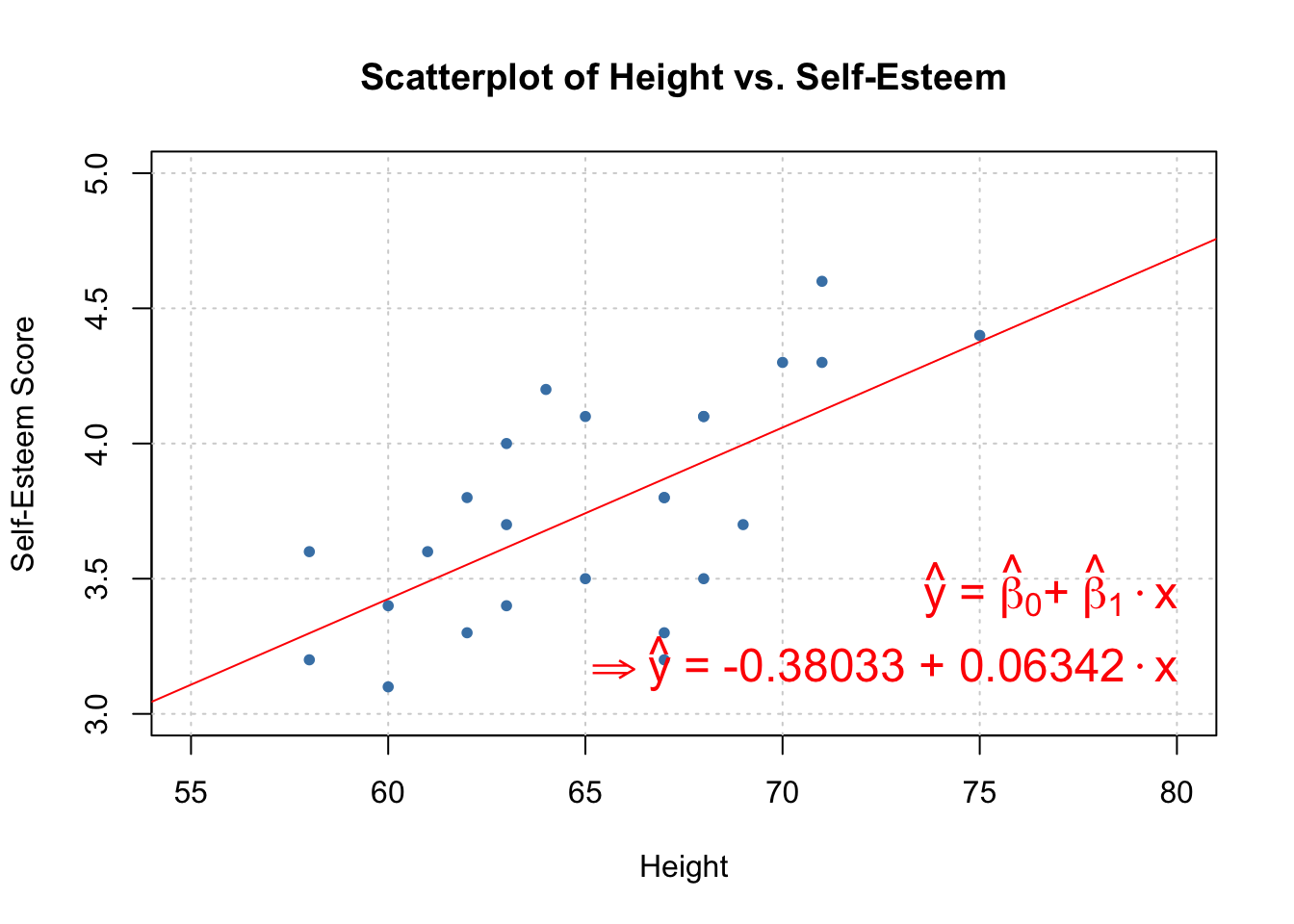
# Determine least-squares regression equation.
m <- lm(data$selfesteem ~ data$height)
# Add this regression line to the scatterplot above.
plot(data$height, data$selfesteem, main = "Scatterplot of Height vs. Self-Esteem",
xlab = "Height", ylab = "Self-Esteem Score", type = "n",
xlim = c(55, 80), ylim = c(3, 5))
grid()
points(data$height, data$selfesteem, col = "steelblue", pch = 20)
abline(m, col = "red")
mtext(expression(paste(hat(y), " = ", hat(beta), ""[0], "+ ", hat(beta), ""[1] %.% x, " ")),
side = 1, col = "red", outer = FALSE, adj = 1, line = -4, cex = 1.5)
mtext(expression(paste(""%=>%hat(y), " = -0.38033 + 0.06342"%.% x," ")),
side = 1, col = "red", outer = FALSE, adj = 1, line = -2, cex = 1.5)
# Question 6
# Display the ANOVA and summary tables to determine test statistic metrics.
anova(m)
## Analysis of Variance Table
##
## Response: data$selfesteem
##             Df Sum Sq Mean Sq F value    Pr(>F)
## data$height  1 1.8063 1.80632  17.071 0.0004054 ***
## Residuals   23 2.4337 0.10581
## ---
## Signif. codes:  0 '***' 0.001 '**' 0.01 '*' 0.05 '.' 0.1 ' ' 1
summary(m)
##
## Call:
## lm(formula = data$selfesteem ~ data$height)
##
## Residuals:
##      Min       1Q   Median       3Q      Max
## -0.66909 -0.24224  0.02352  0.24064  0.52118
##
## Coefficients:
##             Estimate Std. Error t value Pr(>|t|)
## (Intercept) -0.38033    1.00420  -0.379 0.708353
## data$height  0.06342    0.01535   4.132 0.000405 ***
## ---
## Signif. codes:  0 '***' 0.001 '**' 0.01 '*' 0.05 '.' 0.1 ' ' 1
##
## Residual standard error: 0.3253 on 23 degrees of freedom
## Multiple R-squared:  0.426,  Adjusted R-squared:  0.4011
## F-statistic: 17.07 on 1 and 23 DF,  p-value: 0.0004054
# Display 90% confidence interval.
confint(m, level = 0.90)
##                     5 %       95 %
## (Intercept) -2.10139508 1.34073233
## data$height  0.03711525 0.08973314
# Load libraries.
library(ggplot2)
# Read and store couple data from Excel document.
couple.data <- read.xlsx("HW3extracredit.xlsx", sheetName = "Sheet1", header = TRUE) ; couple.data
##   Couple Age.of.Wife Age.of.Husband
## 1      1          20             20
## 2      2          30             32
## 3      3          24             22
## 4      4          28             26
## 5      5          28             30
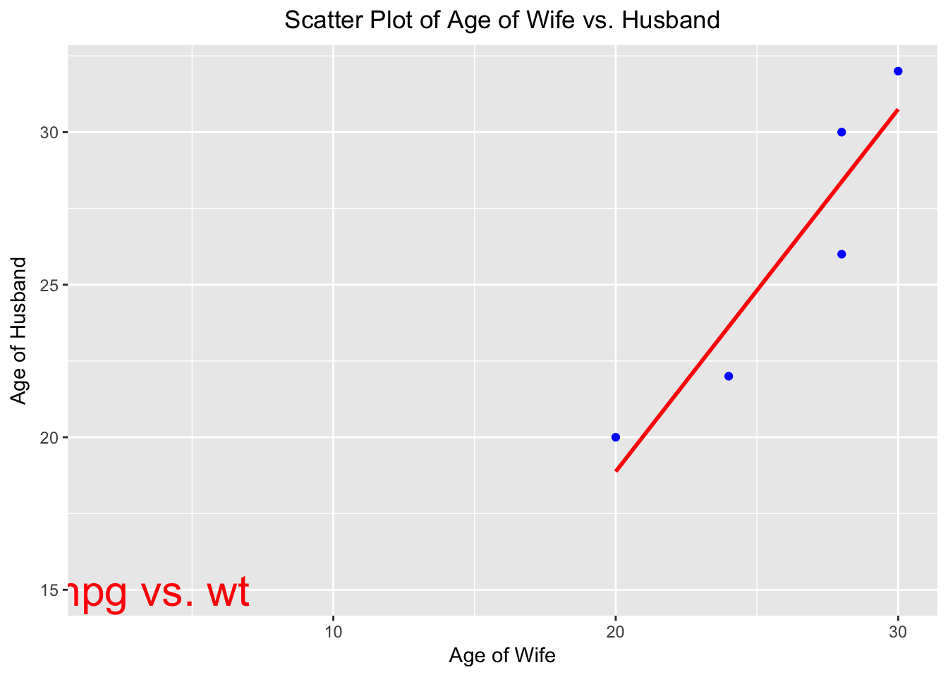
# Draw scatterplot of couple.data.
ggplot(couple.data, aes(x = Age.of.Wife, y = Age.of.Husband)) +
  geom_point(colour = "blue") +
  stat_smooth(method = lm, se = FALSE, colour = "red") +
  labs(x = "Age of Wife", y = "Age of Husband", title = "Scatter Plot of Age of Wife vs. Husband") +
  theme(plot.title = element_text(hjust = 0.5)) +
  annotate("text", label = "plot mpg vs. wt", x = 2, y = 15, size = 8, colour = "red")
# Export plot as PNG image.
ggsave("couplePlot.png", width = 23.8, height = 13.2, unit = "cm", dpi = 300)