# Install and load libraries.
library(xlsx)
## Loading required package: rJava
## Loading required package: xlsxjars
library(plyr)
# Import data from 'homework5data.xlsx' using xlsx function.
iq.data <- read.xlsx("homework5data.xlsx", sheetName = "Sheet1", header = TRUE)

# View summary of iq.data.
summary(iq.data)
##                group          iq             age
##  Chemistry student:15   Min.   :20.00   Min.   :14.00
##  Maths student    :15   1st Qu.:36.00   1st Qu.:17.00
##  Physics student  :15   Median :40.00   Median :18.00
##                         Mean   :39.96   Mean   :26.13
##                         3rd Qu.:46.00   3rd Qu.:40.00
##                         Max.   :52.00   Max.   :58.00
#----------
# Question 1.
#----------
# Determine the number of students in each group.
table(iq.data$group)
##
## Chemistry student     Maths student   Physics student
##                15                15                15
# Determine if 'group' is a factor; if 'true', proceed ; otherwise, create factor.
is.factor(iq.data$group)
## [1] TRUE
# Summarize data relating to IQ score by group of students.
ddply(iq.data, "group", summarise,
      N = length(iq),
      mean = mean(iq),
      sd = sd(iq))
##               group  N     mean       sd
## 1 Chemistry student 15 48.20000 2.396426
## 2     Maths student 15 35.86667 6.937133
## 3   Physics student 15 35.80000 7.793770
# Summarize data relating to age by group of students.
ddply(iq.data, "group", summarise,
      N = length(age),
      mean = mean(age),
      sd = sd(age))
##               group  N     mean       sd
## 1 Chemistry student 15 44.33333 6.651172
## 2     Maths student 15 17.33333 1.046536
## 3   Physics student 15 16.73333 1.437591
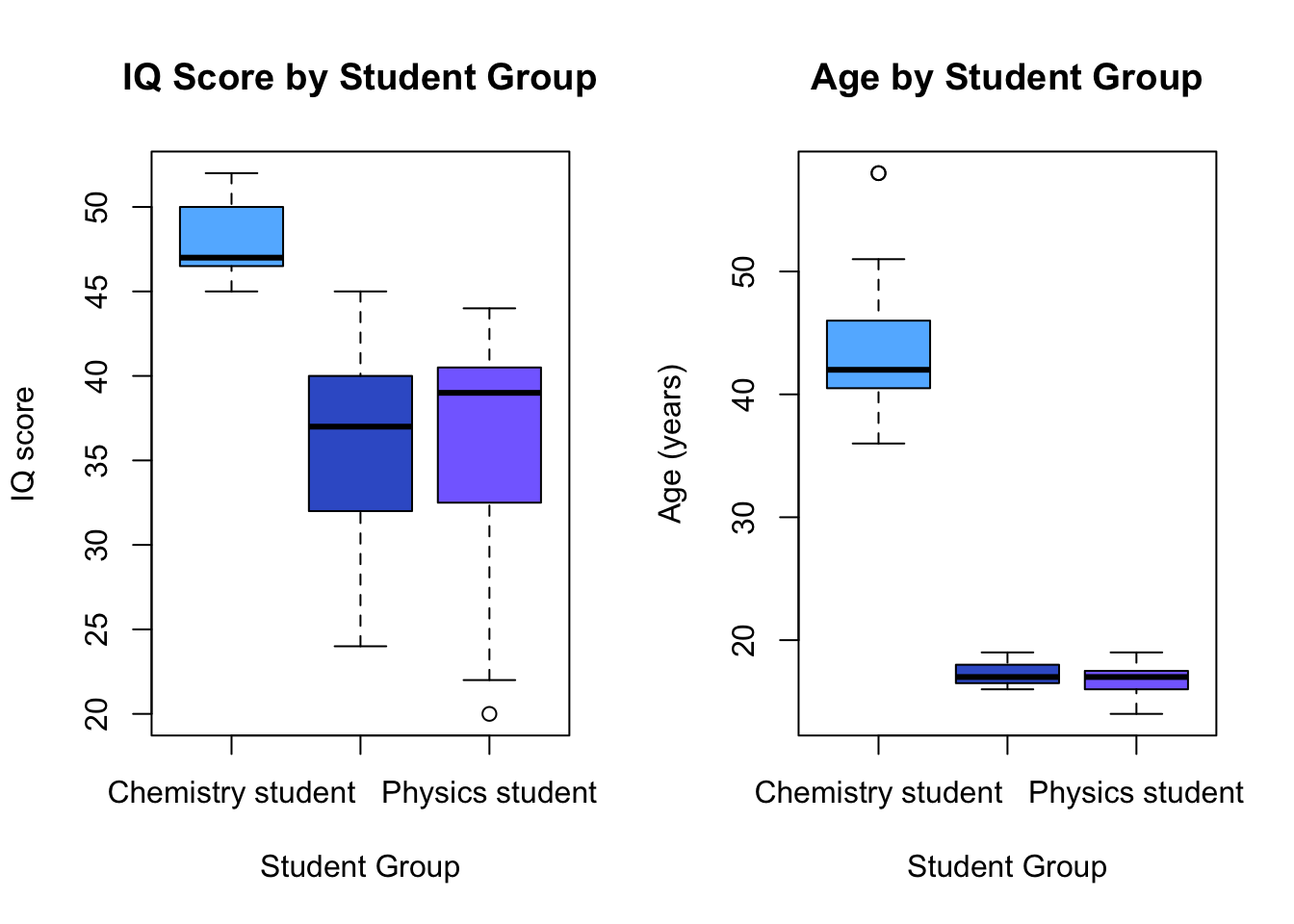
# Generate boxplots for each group.
par(mfrow = c(1, 2))     # Set par settings for two side-by-side plots
boxplot(iq.data$iq ~ iq.data$group, data = iq.data,
        main = "IQ Score by Student Group", ylab = "IQ score",
        xlab = "Student Group",
        col = c("steelblue1", "royalblue3", "lightslateblue"))
boxplot(iq.data$age ~ iq.data$group, data = iq.data,
        main = "Age by Student Group", ylab = "Age (years)",
        xlab = "Student Group",
        col = c("steelblue1", "royalblue3", "lightslateblue"))
par(mfrow = c(1, 1)) # Reset par settings
#----------
# Question 2.
#----------
# Calculate F-statistic to compare against.
qf(0.95, df1 = 2, df2 = 12)
## [1] 3.885294
# Perform a one-way ANOVA for IQ scores.
m <- aov(iq.data$iq ~ iq.data$group) ; m
## Call:
##    aov(formula = iq.data$iq ~ iq.data$group)
##
## Terms:
##                 iq.data$group Residuals
## Sum of Squares       1529.378  1604.533
## Deg. of Freedom             2        42
##
## Residual standard error: 6.180872
## Estimated effects may be unbalanced
summary(m)
##               Df Sum Sq Mean Sq F value   Pr(>F)
## iq.data$group  2   1529   764.7   20.02 7.84e-07 ***
## Residuals     42   1604    38.2
## ---
## Signif. codes:  0 '***' 0.001 '**' 0.01 '*' 0.05 '.' 0.1 ' ' 1
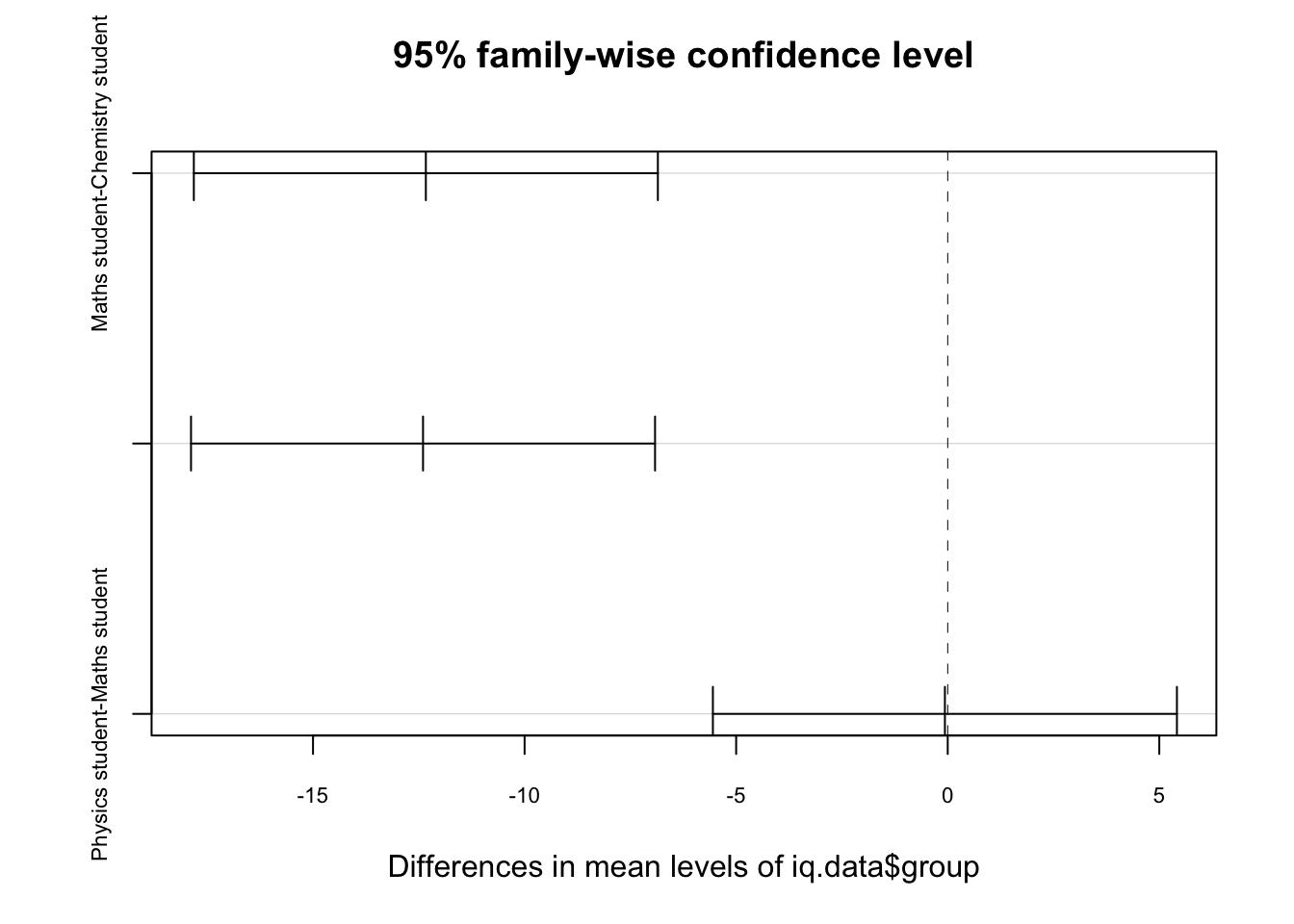
# Perform Tukey's procedure. Display mean diff. conf. intervals.
TukeyHSD(m)
##   Tukey multiple comparisons of means
##     95% family-wise confidence level
##
## Fit: aov(formula = iq.data$iq ~ iq.data$group)
##
## $`iq.data$group`
##                                           diff        lwr       upr
## Maths student-Chemistry student   -12.33333333 -17.816543 -6.850123
## Physics student-Chemistry student -12.40000000 -17.883210 -6.916790
## Physics student-Maths student      -0.06666667  -5.549877  5.416543
##                                       p adj
## Maths student-Chemistry student   0.0000069
## Physics student-Chemistry student 0.0000062
## Physics student-Maths student     0.9995191
plot(TukeyHSD(m), cex.axis = 0.7)
#----------
# Question 3
#----------
# Create dummy variables for student group (chemistry is reference).
iq.data$g.maths <- ifelse(iq.data$group == "Maths student", 1, 0)
iq.data$g.maths
##  [1] 0 0 0 0 0 0 0 0 0 0 0 0 0 0 0 1 1 1 1 1 1 1 1 1 1 1 1 1 1 1 0 0 0 0 0
## [36] 0 0 0 0 0 0 0 0 0 0
iq.data$g.phys <- ifelse(iq.data$group == "Physics student", 1, 0)
iq.data$g.phys
##  [1] 1 1 1 1 1 1 1 1 1 1 1 1 1 1 1 0 0 0 0 0 0 0 0 0 0 0 0 0 0 0 0 0 0 0 0
## [36] 0 0 0 0 0 0 0 0 0 0
head(iq.data) ; tail(iq.data)
##             group iq age g.maths g.phys
## 1 Physics student 44  15       0      1
## 2 Physics student 40  17       0      1
## 3 Physics student 44  15       0      1
## 4 Physics student 39  14       0      1
## 5 Physics student 25  19       0      1
## 6 Physics student 37  18       0      1
##                group iq age g.maths g.phys
## 40 Chemistry student 47  44       0      0
## 41 Chemistry student 46  46       0      0
## 42 Chemistry student 45  38       0      0
## 43 Chemistry student 50  58       0      0
## 44 Chemistry student 47  41       0      0
## 45 Chemistry student 49  42       0      0
# Perform one-way ANOVA test using lm function (including dummies).
m2 <- lm(iq.data$iq ~ iq.data$g.maths + iq.data$g.phys)
summary(m2)
##
## Call:
## lm(formula = iq.data$iq ~ iq.data$g.maths + iq.data$g.phys)
##
## Residuals:
##     Min      1Q  Median      3Q     Max
## -15.800  -2.200   1.133   3.800   9.133
##
## Coefficients:
##                 Estimate Std. Error t value Pr(>|t|)
## (Intercept)       48.200      1.596  30.203  < 2e-16 ***
## iq.data$g.maths  -12.333      2.257  -5.465 2.33e-06 ***
## iq.data$g.phys   -12.400      2.257  -5.494 2.11e-06 ***
## ---
## Signif. codes:  0 '***' 0.001 '**' 0.01 '*' 0.05 '.' 0.1 ' ' 1
##
## Residual standard error: 6.181 on 42 degrees of freedom
## Multiple R-squared:  0.488,  Adjusted R-squared:  0.4636
## F-statistic: 20.02 on 2 and 42 DF,  p-value: 7.843e-07
#----------
# Question 4
#----------
# Re-run ANOVA adjusting for age using Anova function.
require(car)
## Loading required package: car
## Warning: package 'car' was built under R version 3.4.4
## Loading required package: carData
## Warning: package 'carData' was built under R version 3.4.4
options(contrasts = c("contr.treatment", "contr.poly"))
Anova(lm(iq.data$iq ~ iq.data$group + iq.data$age), type = 3)
## Anova Table (Type III tests)
##
## Response: iq.data$iq
##                Sum Sq Df F value    Pr(>F)
## (Intercept)    740.02  1 18.9123 8.842e-05 ***
## iq.data$group  114.82  2  1.4672    0.2424
## iq.data$age      0.25  1  0.0064    0.9367
## Residuals     1604.28 41
## ---
## Signif. codes:  0 '***' 0.001 '**' 0.01 '*' 0.05 '.' 0.1 ' ' 1
# Generate Least Squares means.
require(lsmeans)
## Loading required package: lsmeans
## The 'lsmeans' package is being deprecated.
## Users are encouraged to switch to 'emmeans'.
## See help('transition') for more information, including how
## to convert 'lsmeans' objects and scripts to work with 'emmeans'.
options(contrasts = c("contr.treatment", "contr.poly"))
lsmeans(lm(iq.data$iq ~ iq.data$group + iq.data$age),
        pairwise ~ iq.data$group, adjust = "none")
## $lsmeans
##  iq.data$group       lsmean       SE df lower.CL upper.CL
##  Chemistry student 35.76639 1.669056 41 32.39567 39.13712
##  Maths student     35.80517 1.616411 41 32.54076 39.06958
##  Physics student   35.76639 1.669056 41 32.39567 39.13712
##
## Confidence level used: 0.95
##
## $contrasts
##  contrast                               estimate        SE df t.ratio
##  Chemistry student - Maths student   -0.03877838 0.4856523 41   -0.08
##  Chemistry student - Physics student  0.00000000 0.0000000 41     NaN
##  Maths student - Physics student      0.03877838 0.4856523 41    0.08
##  p.value
##   0.9367
##      NaN
##   0.9367