Distributions
Part 1 - Binomial Distribution
Suppose a pitcher in baseball has 50% chance of getting a strike-out. We want to use the binomial distribution to compute several things.
First, we want to compute the probability distribution for striking out the next six batters. Let’s also plot these probabilities.
# Assign variables and values using the number of batters and probability of a strike-out.
n <- 6 ; p <- 0.5
# Compute the probability of striking out the next six batters.
dbinom(0:n, size = n, prob = p)
## [1] 0.015625 0.093750 0.234375 0.312500 0.234375 0.093750 0.015625# Plot the probability distribution for striking out the next six batters.
heights <- dbinom(0:n, size = n, prob = p)
plot(0:n, heights, type = "h", main = "Spike Plot of X", xlab = "X", ylab = "PMF")
points(0:n, heights, pch = 16)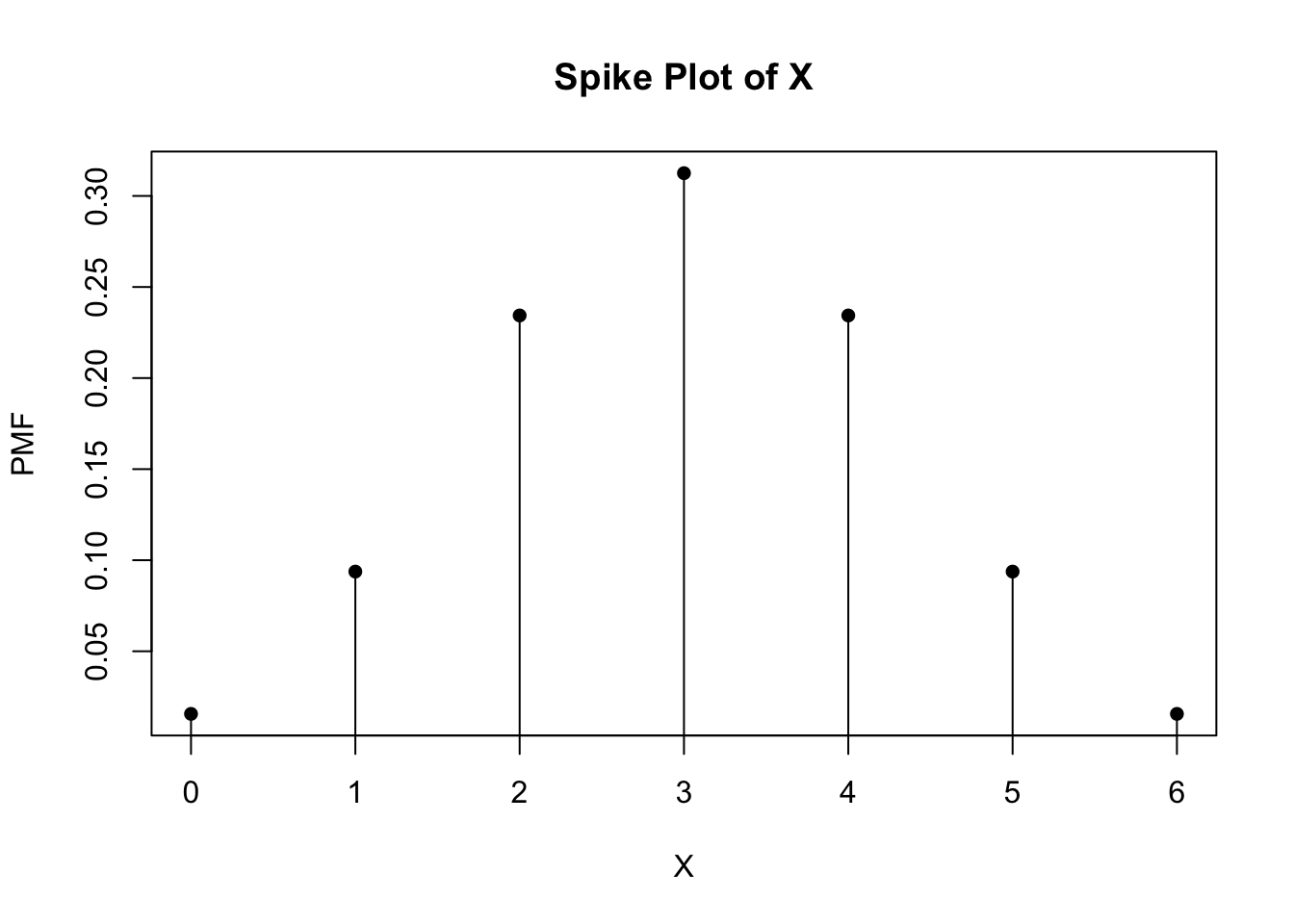
Next, we want to see what the cumulative probabilities look like; the resulting CDF, or cumulative distribution function, plot appears below.
# Assign the binomial distribution to the variable pmf.
pmf <- dbinom(0:n, size = n, prob = p)
# Assign the cumulative distribution function to variable cdf.
cdf <- c(0, cumsum(pmf))
# Assign the step function to the variable cdfplot.
cdfplot <- stepfun(0:n, cdf)
# Display the CDF for the above, ignoring the vertical lines at each step.
plot(cdfplot, verticals = FALSE, pch = 16, main = "Step Plot", xlab = "X", ylab = "CDF")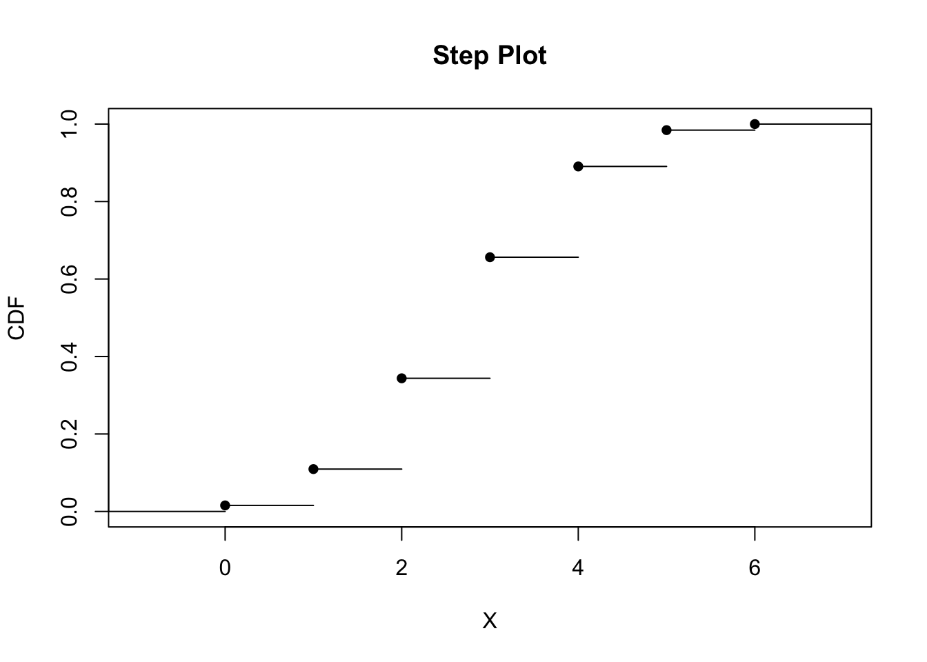
What happens to the probabilities if the pitcher has a 70% chance of getting a strike-out? We can perform the same operations as above but with a p value of 0.7.
# Assign variables and values using the number of batters and probability of a strike-out.
n <- 6 ; p <- 0.7
# Compute the probability of striking out the next six batters.
dbinom(0:n, size = n, prob = p)
## [1] 0.000729 0.010206 0.059535 0.185220 0.324135 0.302526 0.117649# Plot the probability distribution for striking out the next six batters.
heights <- dbinom(0:n, size = n, prob = p)
plot(0:n, heights, type = "h", main = "Spike Plot of X", xlab = "X", ylab = "PMF")
points(0:n, heights, pch = 16)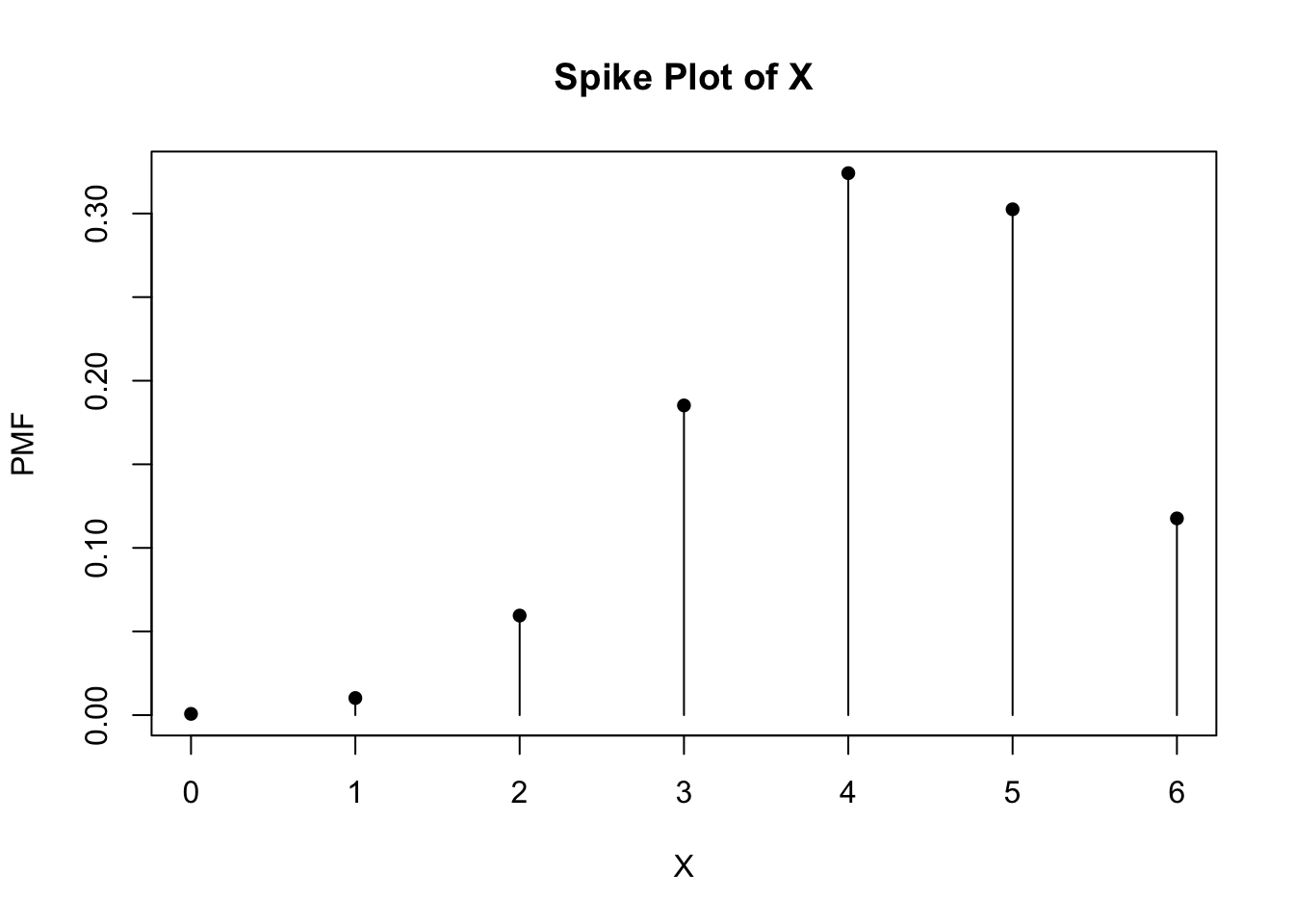
# Assign the binomial distribution to the variable pmf.
pmf <- dbinom(0:n, size = n, prob = p)
# Assign the cumulative distribution function to variable cdf.
cdf <- c(0, cumsum(pmf))
# Assign the step function to the variable cdfplot.
cdfplot <- stepfun(0:n, cdf)
# Display the CDF for the above, ignoring the vertical lines at each step.
plot(cdfplot, verticals = FALSE, pch = 16, main = "Step Plot", xlab = "X", ylab = "CDF")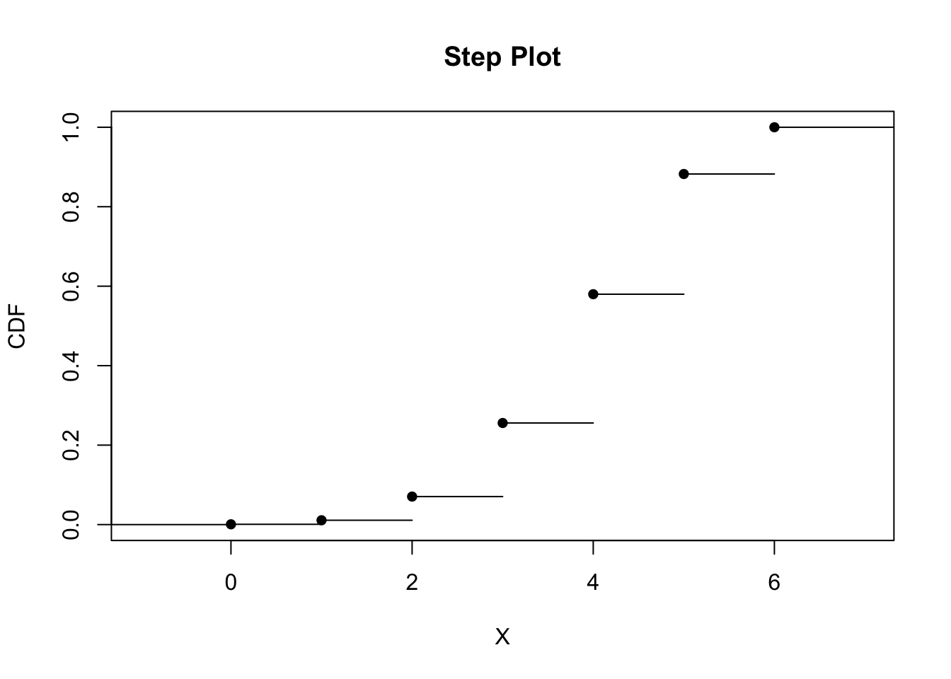
Let’s do the same thing with a probability of the pitcher getting a strike-out at 30%.
# Assign variables and values using the number of batters and probability of a strike-out.
n <- 6 ; p <- 0.3
# Compute the probability of striking out the next six batters.
dbinom(0:n, size = n, prob = p)
## [1] 0.117649 0.302526 0.324135 0.185220 0.059535 0.010206 0.000729# Plot the probability distribution for striking out the next six batters.
heights <- dbinom(0:n, size = n, prob = p)
plot(0:n, heights, type = "h", main = "Spike Plot of X", xlab = "X", ylab = "PMF")
points(0:n, heights, pch = 16)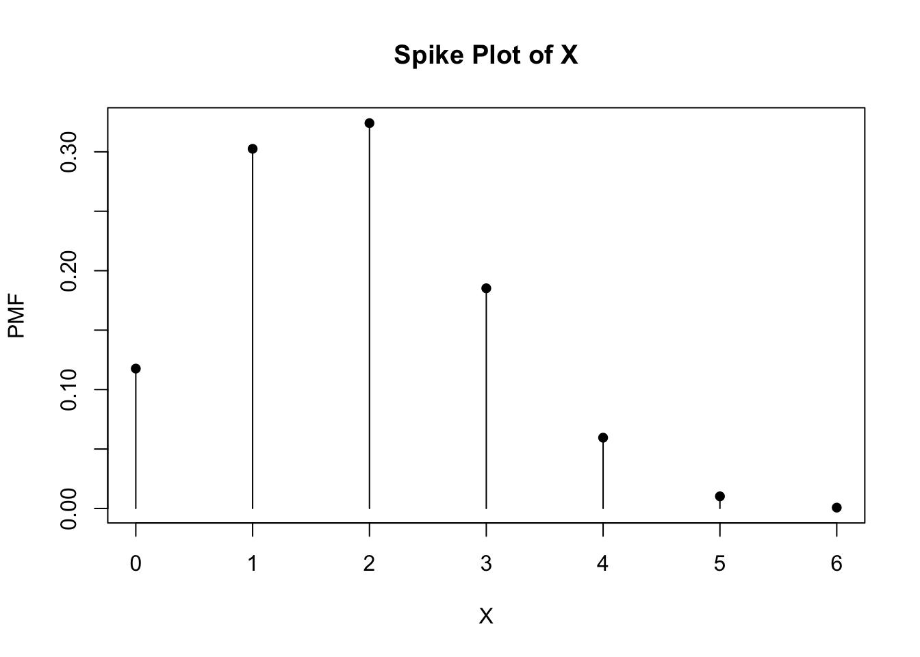
# Assign the binomial distribution to the variable pmf.
pmf <- dbinom(0:n, size = n, prob = p)
# Assign the cumulative distribution function to variable cdf.
cdf <- c(0, cumsum(pmf))
# Assign the step function to the variable cdfplot.
cdfplot <- stepfun(0:n, cdf)
# Display the CDF for the above, ignoring the vertical lines at each step.
plot(cdfplot, verticals = FALSE, pch = 16, main = "Step plot", xlab = "X", ylab = "CDF")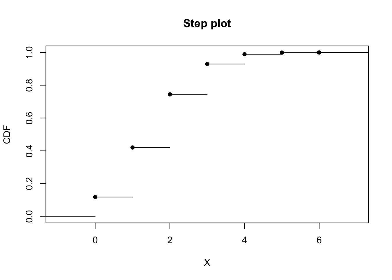
Using the information from the distributions with different probabilities, we can make some inferences from their shapes. When the probability for a pitcher of getting a strike-out is 50%, the probability distribution is symmetrical. The probabilities are evenly distributed around the average number of batters, where the highest probabilty of a strike-out occurs. Here, the average number of batters occurs at (n)(p) = (6)(0.5) = 3. Based on the CDF, the cumulative probabilities increase at a symmetric rate around the inflection point of 3. When the probabilty for a pitcher of getting a strike-out increases to 70%, the probabilty distribution is no longer symmetrical. Instead, it becomes left-skewed, where the bulk of higher probabilities of strike-outs occurs as the number of batters increases. The average number of batters (and thus, highest probability of strike-out) is (n)(p) = (6)(0.7) = 4.2 ~ 4. The CDF shows that the probabilities increase slowly until the inflection point at x = 4 and then increases faster thereafter. When the probability for a pitcher of getting a strike-out decreases to 30%, the probability distribution skews rightward. Here, the bulk of higher probabilities for strike-outs occurs when the number of batters is lower. According to the CDF, the probabilities increase faster until it reaches the average number of batters for strike-out: (n)(p) = (6)(0.3) = 1.8 ~ 2. After x = 2, the probabilites increase at a slower rate.
Part 2 - Binomial Distribution, Continued
Now, suppose that 80% of the flights for an airline arrive on time. We can use the binomial distribution to compute the probability that four flights will arrive on time in the next 10 flights.
# Assign the value of the number of total flights to n and probability of on-time flights to p.
n <- 10; p <- 0.8
# Compute probability of four flights arriving on time in next ten flights.
dbinom(4, size = n, prob = p)
## [1] 0.005505024We can also calculate the probability that four or fewer flights will arrive on time in the next 10 flights.
# Compute probability of four or fewer flights (P(flights <= 4)) will arrive on time in next ten flights.
sum(dbinom(0:4, size = n, prob = p))
## [1] 0.006369382# Display probability of four or fewer flights arriving on time using alternative method.
pbinom(4, size = n, prob = p)## [1] 0.006369382Let’s compute the distribution of probabilities for a flight arriving in time for the next 10 flights.
# Compute probability distribution for flights arriving in time for the next ten flights.
dbinom(0:10, size = n, prob = p)
## [1] 0.0000001024 0.0000040960 0.0000737280 0.0007864320 0.0055050240
## [6] 0.0264241152 0.0880803840 0.2013265920 0.3019898880 0.2684354560
## [11] 0.1073741824# Verify all probabilities are calculated by taking sum of probabilities and verifying it equals one.
sum(dbinom(0:10, size = n, prob = p))## [1] 1Now, let’s display the PMF and CDF for the next 10 flights.
# Display the PMF for the next ten flights.
heights <- dbinom(0:n, size = n, prob = p)
plot(0:n, heights, type = "h", main = "Spike plot of X", xlab = "X", ylab = "PMF")
points(0:n, heights, pch = 16)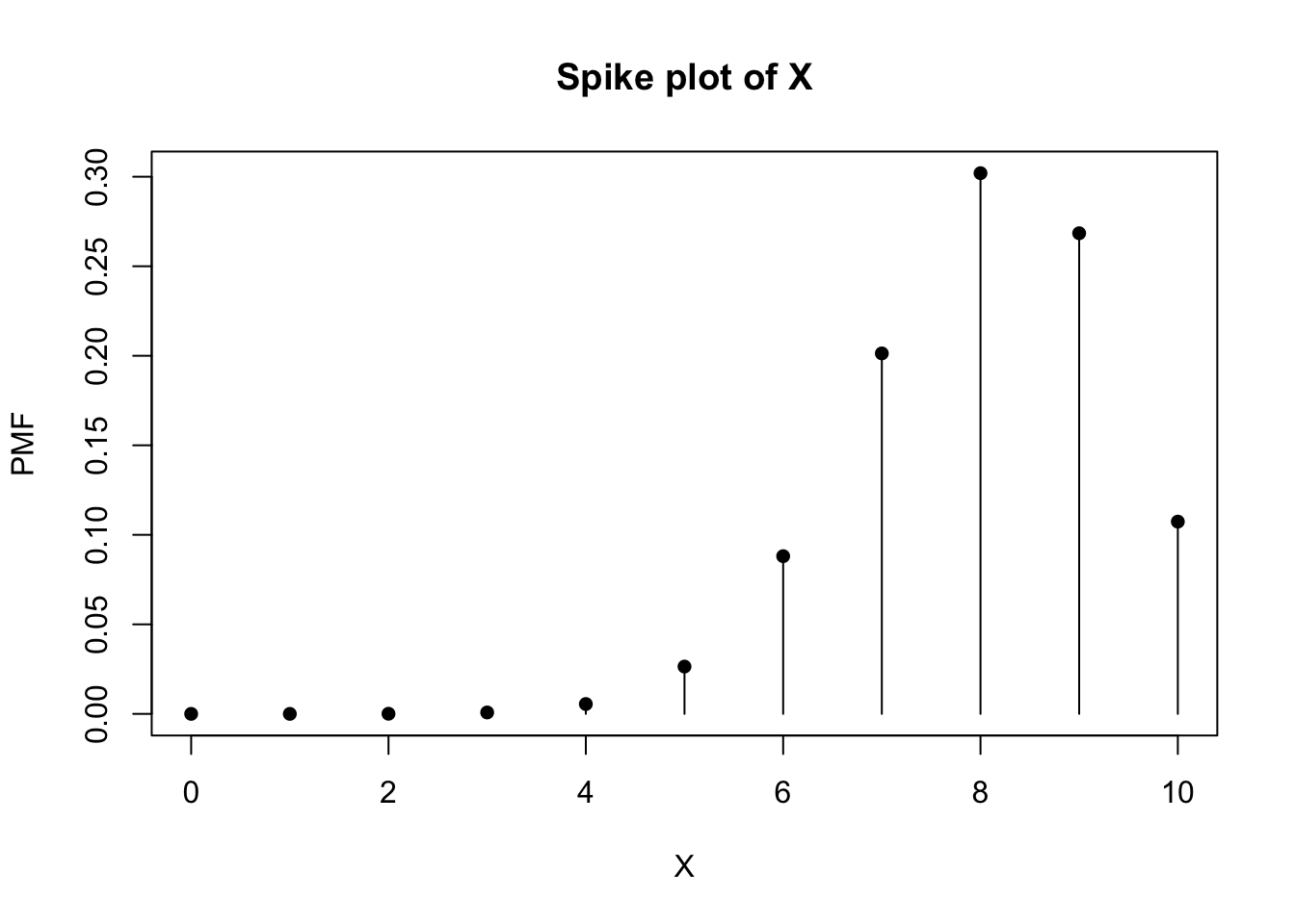
# Display the CDF for the next ten flights.
# Assign the binomial distribution to the variable pmf.
pmf <- dbinom(0:n, size = n, prob = p)
# Assign the cumulative distribution function to variable cdf.
cdf <- c(0, cumsum(pmf))
# Assign the step function to the variable cdfplot.
cdfplot <- stepfun(0:n, cdf)
# Display the CDF for the above, ignoring the vertical lines at each step.
plot(cdfplot, verticals = FALSE, pch = 16, main = "Step plot", xlab = "X", ylab = "CDF")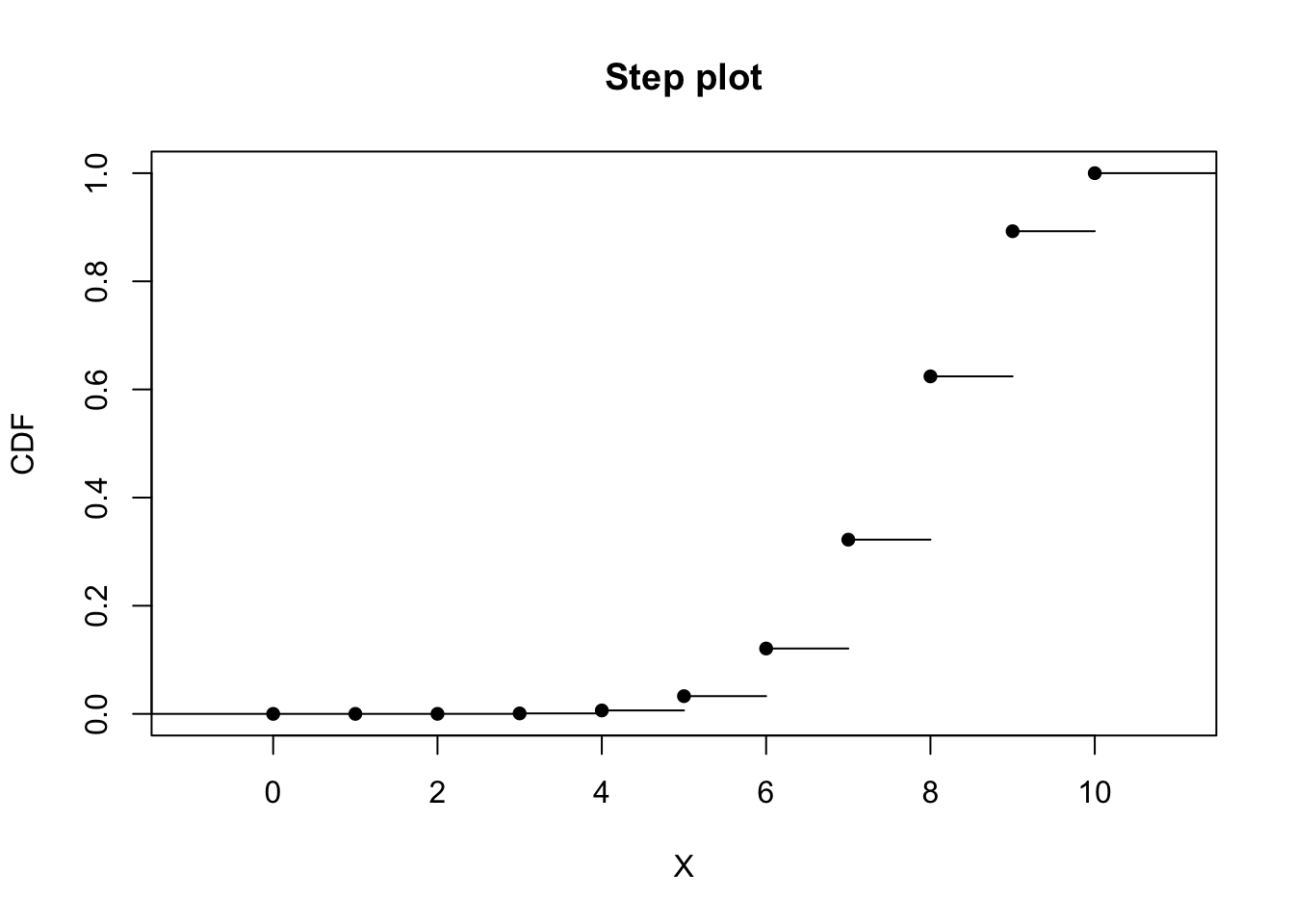
Part 3 - Poisson Distribution
# Compute probability of serving exactly three cars.
dpois(3, lambda = 10)
## [1] 0.007566655# Compute probability of serving at least three cars; P(X >= 3) = 1 - P(X < 3)
1 - ppois(3, lambda = 10)## [1] 0.9896639# Find probabilty of serving between two and five cars.
ppois(5, lambda = 10) - ppois(2, lambda = 10)## [1] 0.06431657# Calculate the PMF for the first 20 cars.
pmf <- dpois(0:20, lambda = 10)
pmf## [1] 4.539993e-05 4.539993e-04 2.269996e-03 7.566655e-03 1.891664e-02
## [6] 3.783327e-02 6.305546e-02 9.007923e-02 1.125990e-01 1.251100e-01
## [11] 1.251100e-01 1.137364e-01 9.478033e-02 7.290795e-02 5.207710e-02
## [16] 3.471807e-02 2.169879e-02 1.276400e-02 7.091109e-03 3.732163e-03
## [21] 1.866081e-03# Display the PMF plot for the first 20 cars.
plot(0:20, pmf, type = "h", xlab = "X", ylab = "PMF")
# Add a red horizontal line at y = 0 for better illustration as an x axis.
abline(h = 0, col = "red")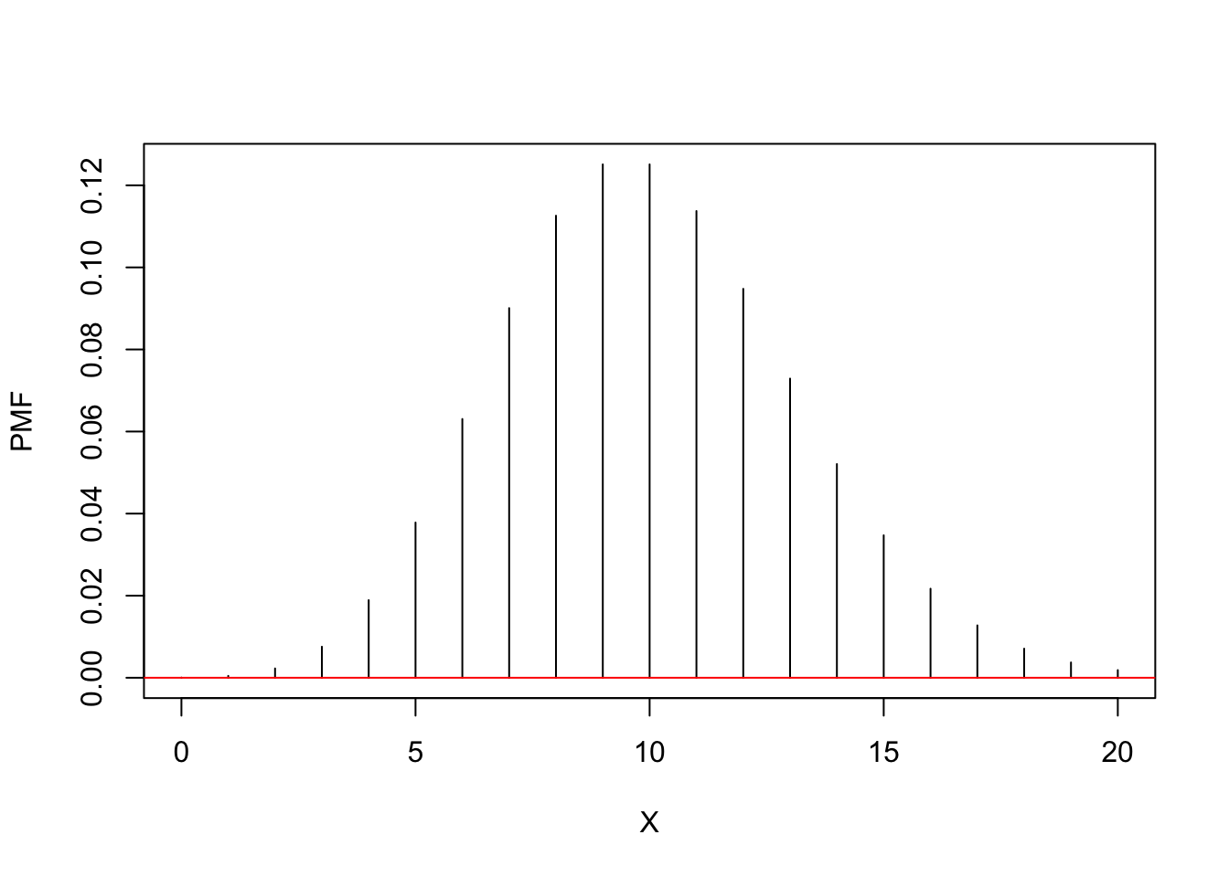
Part 4 - Uniform Distribution
# Assign the range of exam values on the interval [a, b] -> [60, 100] to corresponding variables.
a <- 60; b <- 100
# Use dunif function to find: P(X = 60). Let x = 60.
x <- 60 ; dunif(x, min = a, max = b)
## [1] 0.025# Use dunif function to find: P(X = 80). Let x = 80.
x <- 80 ; dunif(x, min = a, max = b)## [1] 0.025# Use dunif function to find: P(X = 100). Let x = 100.
x <- 100 ; dunif(x, min = a, max = b)## [1] 0.025# Compute the mean of this distribution.
x <- a:b # Create the vector sequence of numbers from 60 to 100; store in x.
f <- rep(1/(length(a:b)), length(a:b)) # Create the probability vector for each x.
mu <- sum(x * f) ; mu # Calculate the mean and store in mu; display the result.## [1] 80# Compute the standard deviation of this distribution.
sigmaSquare <- sum((x - mu)^2 * f) # Calculate the variance of f and store in sigmaSquare.
sqrt(sigmaSquare) # Calculate the std. dev. by taking square root of sigmaSquare## [1] 11.83216# Display the probabilities of scoring between 60 and 70.
pmf <- dunif(a:70, min = a, max = b) ; pmf## [1] 0.025 0.025 0.025 0.025 0.025 0.025 0.025 0.025 0.025 0.025 0.025# Sum the probabilities to find P(X <= 70).
sum(pmf)## [1] 0.275# Calculate probability of scoring greater than 80: P(X > 80).
punif(80, min = a, max = b, lower.tail = FALSE)## [1] 0.5# Calculate probabilty of P(X >= 90).
# Using the lower.tail = FALSE option, we get P(X > 90). Add P(X = 90) so we can get P(X >= 90).
punif(90, min = a, max = b, lower.tail = FALSE)## [1] 0.25Part 5 - Normal Distribution
# Three standard deviations on either side of the mean: [a, b] ~ [100 - 3 * 10, 100 + 3 * 10] = [70, 130]
# Expand range to completely cover [70, 130] -> [50, 150]
# Assign min, max, mean and std. dev. values to variables.
a <- 50 ; b <- 150 ; mu <- 100 ; sigma <- 10
# Create a sequence vector of values from [70, 130].
x <- seq(a, b)
# Create the PDF for x.
pdf <- dnorm(x, mean = mu, sd = sigma)
# Display the normal curve for this distribution.
plot(x, pdf, type = "l", col = "red", xlim = c(a, b), main = "Average $ Spent on Souvenirs",
    xlab = "Dollars Spent ($)", ylab = "PDF")
# Add dashed vertical lines at mean and std. dev. from mean and horizontal line at y = 0 for enhanced visibility.
abline(v = c(mu - 3 * sigma, mu - 2 * sigma, mu - sigma, mu, mu + sigma, mu + 2 * sigma, mu + 3 * sigma),
       col = "light blue", lty = 2) ; abline(h = 0)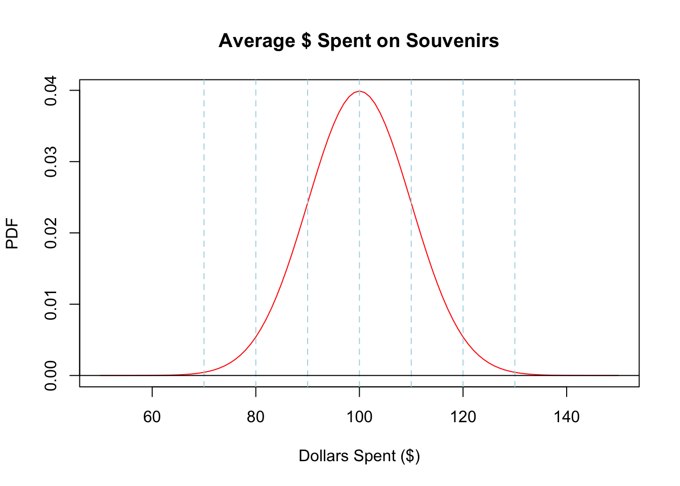
# Calculate P(X > 120): P(X > 120) = 1 - P(X <= 120). Use pnorm to find P(X <= 120).
1 - pnorm(120, mean = mu, sd = sigma)
## [1] 0.02275013# P(80 <= X <= 90) = P(X <= 90) - P(X <= 80).
pnorm(90, mean = mu, sd = sigma) - pnorm(80, mean = mu, sd = sigma)## [1] 0.1359051# Probability of spending within one standard deviation:
pnorm(mu + sigma, mean = mu, sd = sigma) - pnorm(mu - sigma, mean = mu, sd = sigma)## [1] 0.6826895# Probability of spending within two standard deviations:
pnorm(mu + 2 * sigma, mean = mu, sd = sigma) - pnorm(mu - 2 * sigma, mean = mu, sd = sigma)## [1] 0.9544997# Probability of spending within three standard deviations:
pnorm(mu + 3 * sigma, mean = mu, sd = sigma) - pnorm(mu - 3 * sigma, mean = mu, sd = sigma)## [1] 0.9973002# Use qnorm function to find the lower value from which 90% of money spent will fall.
# Using the symmetry of this normal distribution to find lower half of 90%, we can determine that 45% falls
# below the mean, giving us the need to find the value where sum of probabilities equals 50 - 45 = 5%.
lower <- qnorm(0.05, mean = mu, sd = sigma) ; lower## [1] 83.55146# Use qnorm function to find the upper value.
# Again, using the symmetry of the distribution, we determine that another 45% falls above the mean,
# giving us the need to find the value where sum of probabilities equals 50 + 45 = 95%.
upper <- qnorm(0.95, mean = mu, sd = sigma) ; upper## [1] 116.4485# Verify the range of values from above contains the middle 90% of the money spent; if accurate, P = 0.9.
pnorm(upper, mean = mu, sd = sigma) - pnorm(lower, mean = mu, sd = sigma)## [1] 0.9# Generate a vector of random values which follow the normal distribution with
# the mean and std. dev. above. Round the values.
y <- rnorm(10000, mean = mu, sd = sigma)
y <- round(y)
# Display the plot for the randomly generated sample above.
plot(table(y), type = "h", xlab = "Dollars Spent ($)", ylab = "Number of Visitors")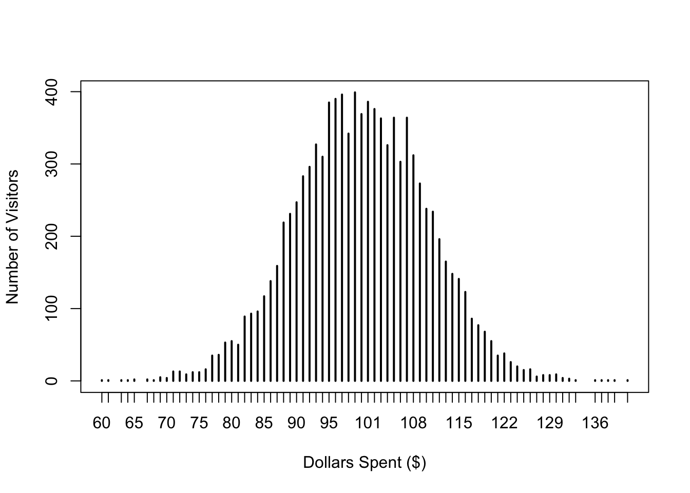
Part 6 - Exponential Distribution
# Let lambda = 18.
lambda <- 18
# P(Call arrives within two minutes) = P(t <= 2/60).
pexp(2/60, rate = lambda)
## [1] 0.4511884# P(Call arrives within five minutes) = P(t <= 5/60).
pexp(5/60, rate = lambda)## [1] 0.7768698# P(Call arrives between two minutes and five minutes) = P(2 <= X <= 5) = P(X <= 5) - P(X <= 2), X = minutes.
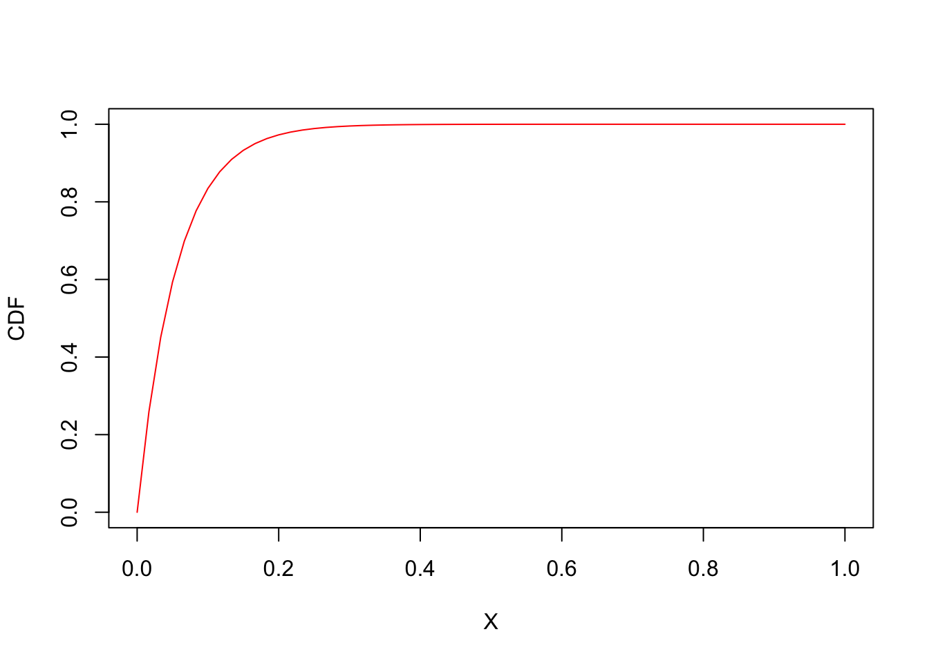
pexp(5/60, rate = lambda) - pexp(2/60, rate = lambda)## [1] 0.3256815# Display the CDF of this distribution.
plot(seq(0, 1, by = 1/60), pexp(seq(0, 1, by = 1/60), rate = lambda),
type = "l", col = "red", xlab = "X", ylab = "CDF")