# Install the "UsingR" package.
# install.packages("UsingR")
# Load the "UsingR" library quietly by suppressing startup message.
# Reference: "Package 'startupmsg'". April 23, 2016. https://cran.r-project.org/web/packages/startupmsg/startupmsg.pdf
suppressPackageStartupMessages(library(UsingR))
## Warning: package 'HistData' was built under R version 3.4.4
library(UsingR)
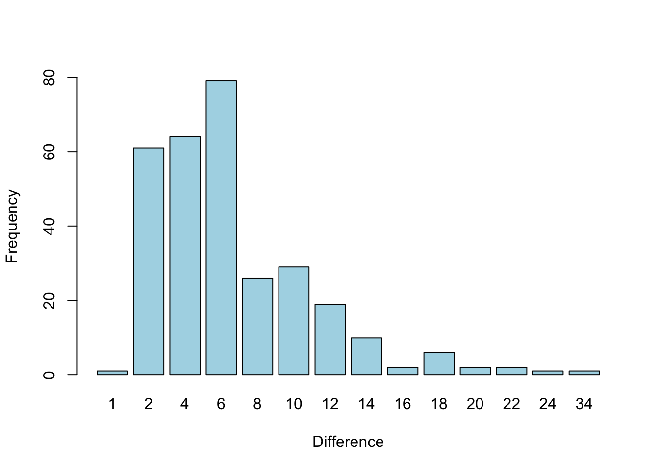
# Use the diff function to compute differences between successive prime numbers.
diff(primes)
##   [1]  1  2  2  4  2  4  2  4  6  2  6  4  2  4  6  6  2  6  4  2  6  4  6
##  [24]  8  4  2  4  2  4 14  4  6  2 10  2  6  6  4  6  6  2 10  2  4  2 12
##  [47] 12  4  2  4  6  2 10  6  6  6  2  6  4  2 10 14  4  2  4 14  6 10  2
##  [70]  4  6  8  6  6  4  6  8  4  8 10  2 10  2  6  4  6  8  4  2  4 12  8
##  [93]  4  8  4  6 12  2 18  6 10  6  6  2  6 10  6  6  2  6  6  4  2 12 10
## [116]  2  4  6  6  2 12  4  6  8 10  8 10  8  6  6  4  8  6  4  8  4 14 10
## [139] 12  2 10  2  4  2 10 14  4  2  4 14  4  2  4 20  4  8 10  8  4  6  6
## [162] 14  4  6  6  8  6 12  4  6  2 10  2  6 10  2 10  2  6 18  4  2  4  6
## [185]  6  8  6  6 22  2 10  8 10  6  6  8 12  4  6  6  2  6 12 10 18  2  4
## [208]  6  2  6  4  2  4 12  2  6 34  6  6  8 18 10 14  4  2  4  6  8  4  2
## [231]  6 12 10  2  4  2  4  6 12 12  8 12  6  4  6  8  4  8  4 14  4  6  2
## [254]  4  6  2  6 10 20  6  4  2 24  4  2 10 12  2 10  8  6  6  6 18  6  4
## [277]  2 12 10 12  8 16 14  6  4  2  4  2 10 12  6  6 18  2 16  2 22  6  8
## [300]  6  4  2  4
# Show the frequencies of the above differences.
table(diff(primes))
##
##  1  2  4  6  8 10 12 14 16 18 20 22 24 34
##  1 61 64 79 26 29 19 10  2  6  2  2  1  1
# Show the barplot of these differences.
barplot(table(diff(primes)), ylim = c(0,80), xlab = "Difference", ylab = "Frequency", col = "lightblue")
# Display first few rows of "coins" dataset as a table of frequencies.
head(table(coins))
##       value
## year   0.01 0.05 0.1 0.25
##   1929    2    1   0    0
##   1936    0    0   1    0
##   1939    0    0   1    0
##   1955    0    0   0    1
##   1959    1    0   0    0
##   1960    1    0   0    0
# Display "coins" dataset as a table of frequencies by denomination, excluding years.
table(coins$value)
##
## 0.01 0.05  0.1 0.25
##  203   59   42   67
# Multiply the sum of coins in each denomination and multiply by denomination.
table(coins$value) * c(as.numeric(levels(factor(coins$value))))
##
##  0.01  0.05   0.1  0.25
##  2.03  2.95  4.20 16.75
# Display the sum of frequency of values in the "coins" table.
sum(coins$value)
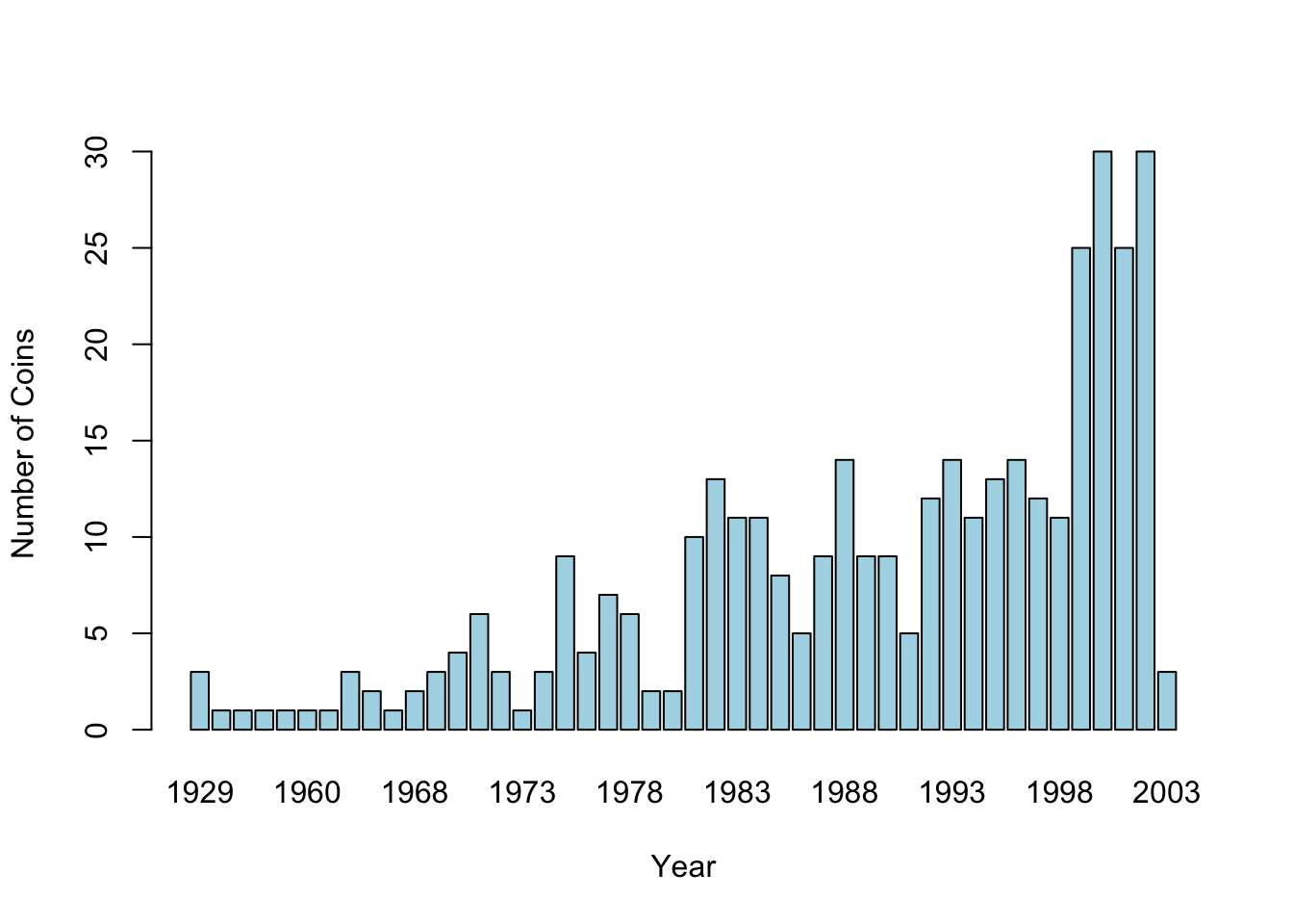
## [1] 25.93
barplot(table(coins$year), xlab = "Year", ylab = "Number of Coins", col = "lightblue")
# Display the first few items of "south" dataset.
head(south)
## [1] 12 10 10 13 12 12
# Display the "south" dataset as a stemplot.
stem(south)
##
##   The decimal point is 1 digit(s) to the right of the |
##
##   0 | 6788
##   1 | 000011122222334444
##   1 | 6688
##   2 | 0
##   2 | 59
##   3 | 3
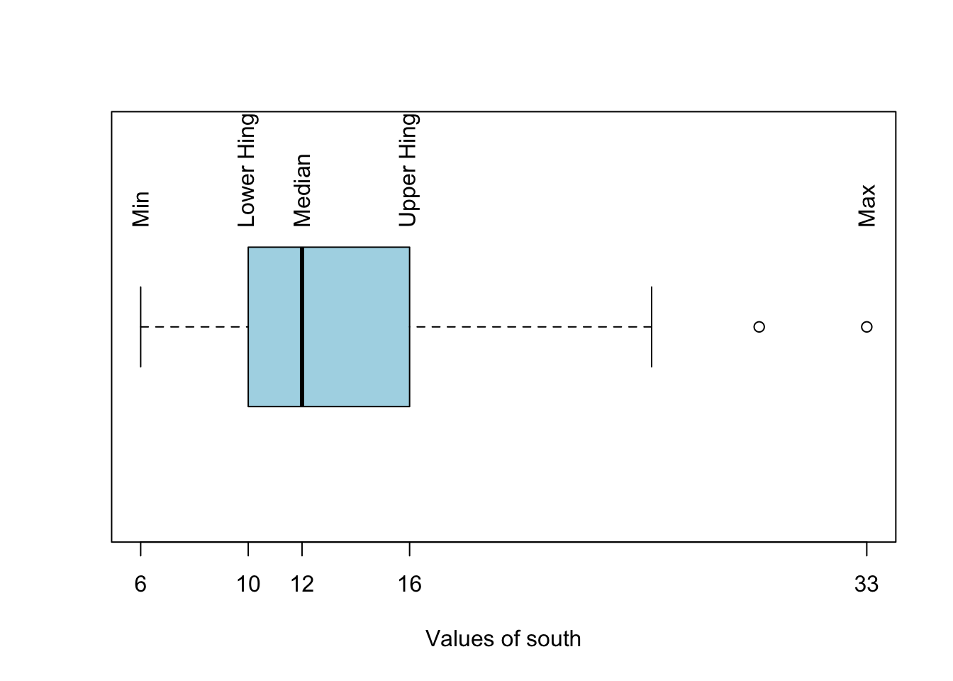
# Display the five-number summary of 'south'.
f <- fivenum(south)
f
## [1] 6 10 12 16 33
# Display the lower and upper outlier range values.
g <- c(f[2] - 1.5*(f[4] - f[2]), f[4] + 1.5*(f[4] - f[2]))
g
## [1] 1 25
# Create a vector containing the values of south which are below the lower outerlier (L)
# and above the upper outerlier (U). Sort the results.
sort(c(south[which(((south > c(g[2])) == TRUE), ((south < c(g[1])) == TRUE))]))
## [1] 29 33
# Show horizontal boxplot of "south".
boxplot(south, horizontal = TRUE, xaxt = "n", xlab = "Values of south", col = "lightblue")

# View the five-number summary of south on x-axis.
axis(side = 1, at = fivenum(south), labels = TRUE)

# Display value representations of five-number summary above boxplot.
text(fivenum(south), rep(1.25, 5), srt=90, adj=0,
    labels = c("Min", "Lower Hinge", "Median", "Upper Hinge", "Max"))
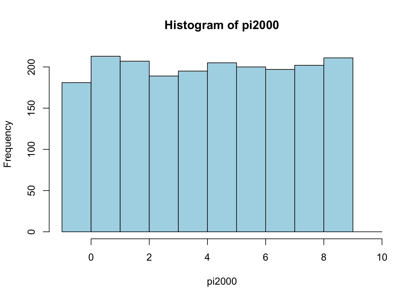
# Display pi2000 as a table, showing frequencies of each digit of the dataset.
table(pi2000)
## pi2000
##   0   1   2   3   4   5   6   7   8   9
## 181 213 207 189 195 205 200 197 202 211
# Divide each value of pi2000 by the length of the pi2000 dataset.
# Multiply the results by 100; results are percentages of their frequencies.
(table(pi2000) / length(pi2000)) * 100
## pi2000
##     0     1     2     3     4     5     6     7     8     9
##  9.05 10.65 10.35  9.45  9.75 10.25 10.00  9.85 10.10 10.55
# Display historgram of pi2000; include breaks to show separate frequency values of 0 and 1.
hist(pi2000, breaks = -1:10, col = "lightblue")
S <- cbind(c(25, 20), c(10, 40), c(15, 30))
S
##      [,1] [,2] [,3]
## [1,]   25   10   15
## [2,]   20   40   30
rownames(S) <- c("Men", "Women")
S
##       [,1] [,2] [,3]
## Men     25   10   15
## Women   20   40   30
colnames(S) <- c("NFL", "NBA", "NHL")
S
##       NFL NBA NHL
## Men    25  10  15
## Women  20  40  30
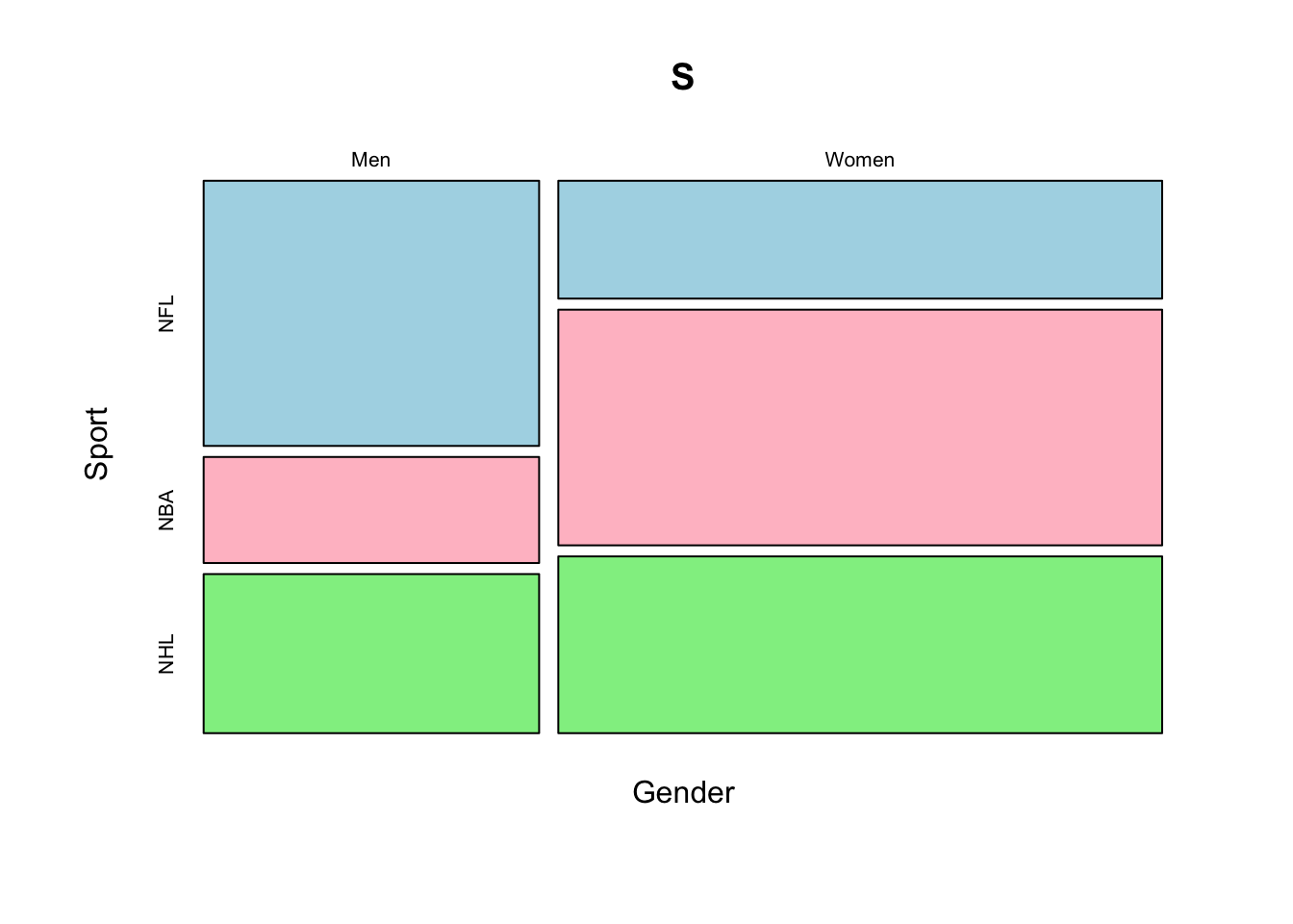
dimnames(S) <- list(Gender = rownames(S), Sport = colnames(S))
dimnames(S)
## $Gender
## [1] "Men"   "Women"
##
## $Sport
## [1] "NFL" "NBA" "NHL"
S
##        Sport
## Gender  NFL NBA NHL
##   Men    25  10  15
##   Women  20  40  30
# Display marginal distributions for Gender.
margin.table(S, 1)
## Gender
##   Men Women
##    50    90
# Display marginal distributions for Sport.
margin.table(S, 2)
## Sport
## NFL NBA NHL
##  45  50  45
addmargins(S)
##        Sport
## Gender  NFL NBA NHL Sum
##   Men    25  10  15  50
##   Women  20  40  30  90
##   Sum    45  50  45 140
# Display proportional data for Gender.
prop.table(S, 1)
##        Sport
## Gender        NFL       NBA       NHL
##   Men   0.5000000 0.2000000 0.3000000
##   Women 0.2222222 0.4444444 0.3333333
# Display proportional data for Sport.
prop.table(S, 2)
##        Sport
## Gender        NFL NBA       NHL
##   Men   0.5555556 0.2 0.3333333
##   Women 0.4444444 0.8 0.6666667
# Display the mosaic plot for the data.
mosaicplot(S, color = c("light blue", "pink", "light green"))
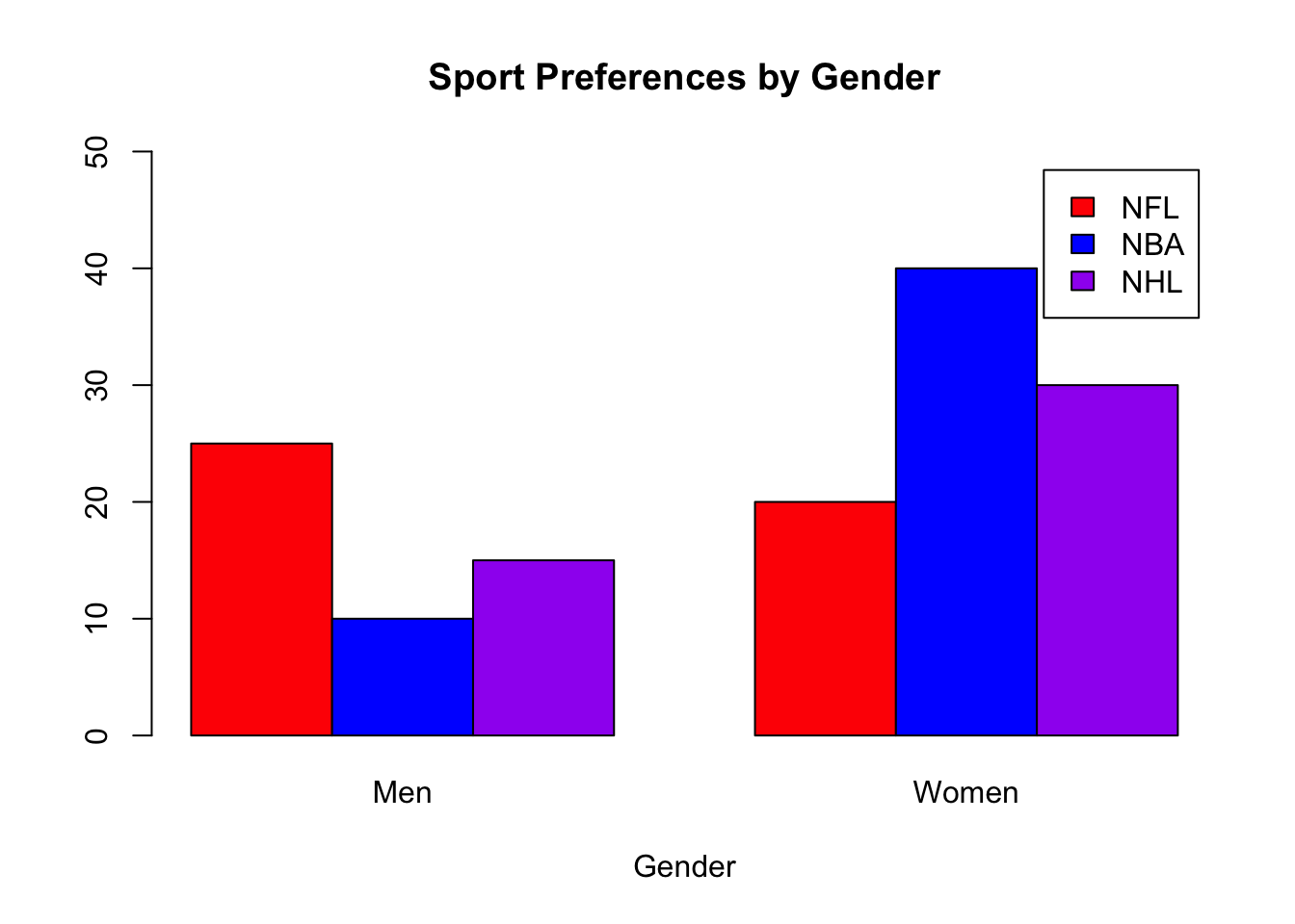
# Display the barplot for Gender.
barplot(t(S), xlab = "Gender", beside = TRUE, legend = TRUE, main = "Sport Preferences by Gender",
        ylim = c(0, 50), col = c("red", "blue", "purple"))
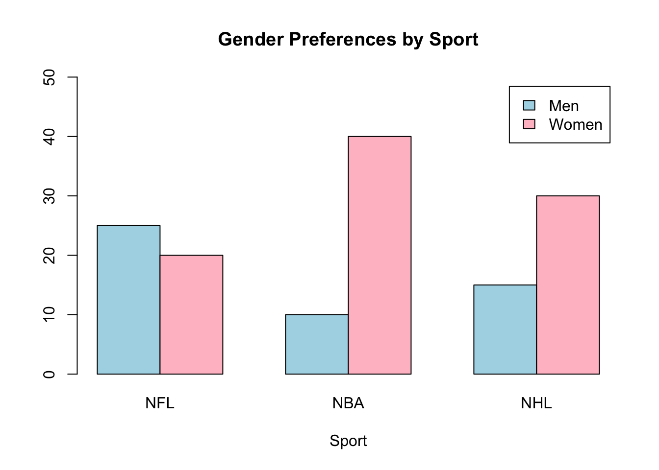
# Display the barplot for Sport.
barplot(S, xlab = "Sport", beside = TRUE, legend = TRUE, main = "Gender Preferences by Sport",
        ylim = c(0, 50), col = c("light blue", "pink"))
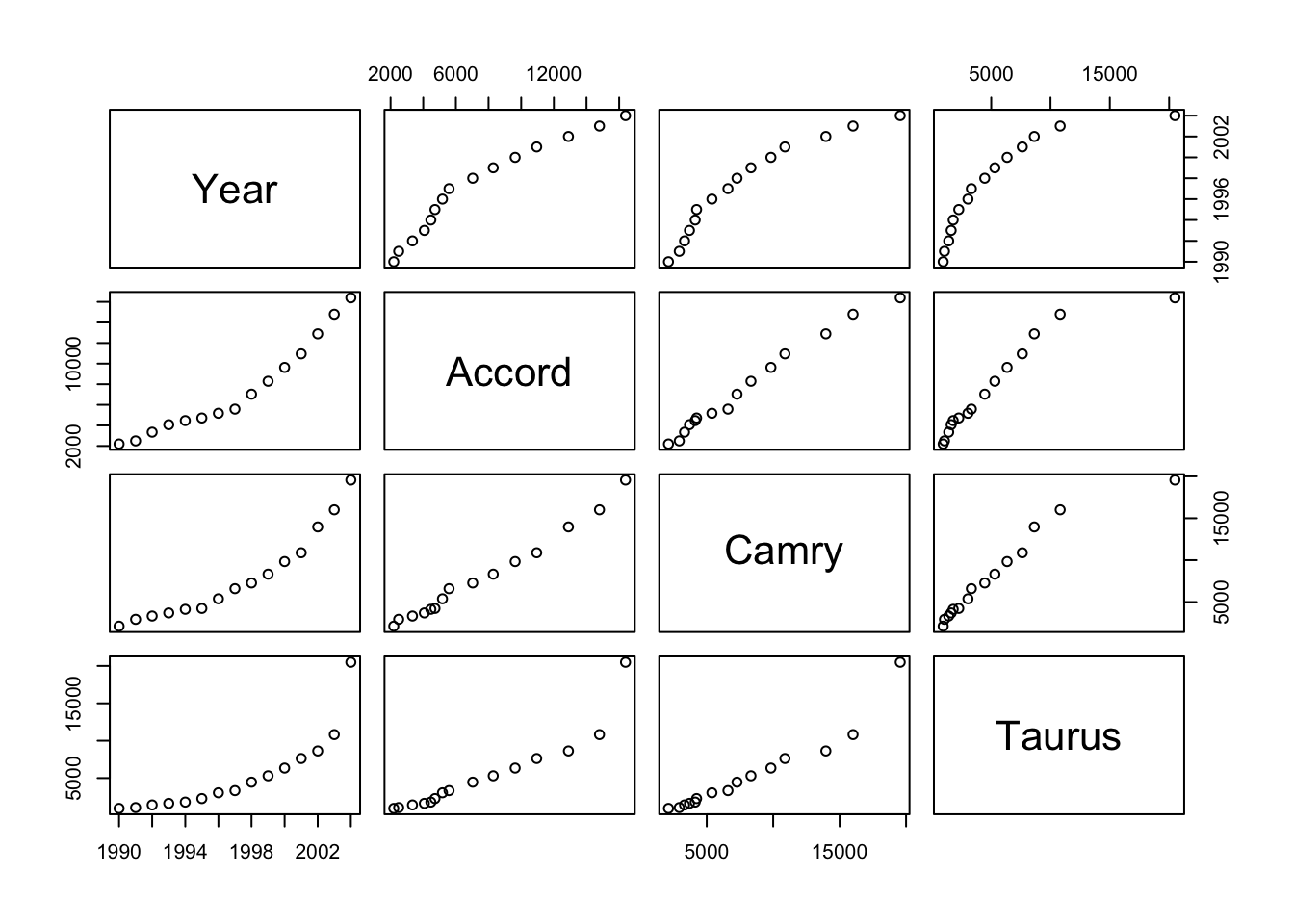
# Display the first few rows of "midsize" dataset.
head(midsize)
##   Year Accord Camry Taurus
## 1 2004  16390 19560  20490
## 2 2003  14795 16010  10817
## 3 2002  12893 13965   8633
## 4 2001  10949 10884   7620
## 5 2000   9630  9830   6340
## 6 1999   8287  8328   5308
# Display a pair-wise plot for "midsize".
pairs(midsize)
# Display the first few rows of "MLBattend" dataset.
head(MLBattend)
##   franchise league division year attendance runs.scored runs.allowed wins
## 1       BAL     AL     EAST   69    1062069         779          517  109
## 2       BOS     AL     EAST   69    1833246         743          736   87
## 3       CLE     AL     EAST   69     619970         573          717   62
## 4       DET     AL     EAST   69    1577481         701          601   90
## 5       NYA     AL     EAST   69    1067996         562          587   80
## 6       WAS     AL     EAST   69     918106         694          644   86
##   losses games.behind
## 1     53          0.0
## 2     75         22.0
## 3     99         46.5
## 4     72         19.0
## 5     81         28.5
## 6     76         23.0
# Store wins values for BAL in "wvBAL"
wvBAL <- c(MLBattend$wins[which(MLBattend$franchise == "BAL")])

# Display wins values vector for BAL.
wvBAL
##  [1] 109 108 101  80  97  91  90  88  97  90 102 100  59  94  98  85  83
## [18]  73  67  54  87  76  67  89  85  63  71  88  98  79  78  74
# Store wins values for BOS in "wvBOS"
wvBOS <- c(MLBattend$wins[which(MLBattend$franchise == "BOS")])

# Display wins values vector for BOS.
wvBOS
##  [1] 87 87 85 85 89 84 95 83 97 99 91 83 59 89 78 86 81 95 78 89 83 88 84
## [24] 73 80 54 86 85 78 92 94 85
# Store wins values for DET in "wvDET"
wvDET <- c(MLBattend$wins[which(MLBattend$franchise == "DET")])

# Display wins values vector for DET.
wvDET
##  [1]  90  79  91  86  85  72  57  74  74  86  85  84  60  83  92 104  84
## [18]  87  98  88  59  79  84  75  85  53  60  53  79  65  69  79
# Store wins values for LA in "wvLA"
wvLA <- c(MLBattend$wins[which(MLBattend$franchise == "LA")])

# Display wins values vector for LA.
wvLA
##  [1]  85  87  89  85  95 102  88  92  98  95  79  92  63  88  91  79  95
## [18]  73  73  94  77  86  93  63  81  58  78  90  88  83  77  86
# Store wins values for PHI in "wvPHI"
wvPHI <- c(MLBattend$wins[which(MLBattend$franchise == "PHI")])

# Display wins values vector for PHI.
wvPHI
##  [1]  63  73  67  59  71  80  86 101 101  90  84  91  59  89  90  81  75
## [18]  86  80  65  67  77  78  70  97  54  69  67  68  75  77  65
# Create a data frame of names and each team's wins
team.info <- data.frame(
                        BAL = wvBAL,
                        BOS = wvBOS,
                        DET = wvDET,
                        LA = wvLA,
                        PHI = wvPHI)

# Display the first few rows of the team.info data frame.
head(team.info)
##   BAL BOS DET  LA PHI
## 1 109  87  90  85  63
## 2 108  87  79  87  73
## 3 101  85  91  89  67
## 4  80  85  86  85  59
## 5  97  89  85  95  71
## 6  91  84  72 102  80
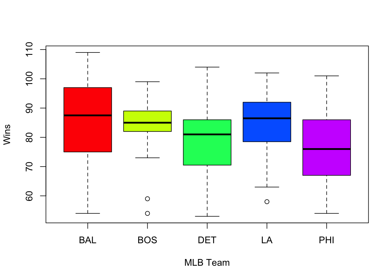
# Display boxplot of team.info data frame.
boxplot(team.info, col = rainbow(5), xlab = "MLB Team", ylab = "Wins")
# Read information from senate.csv and store in "senate".
senate <- read.csv("http://kalathur.com/cs544/data/senate.csv", header = TRUE)
# Display first few rows of "senate".
head(senate)
##             Name Years_in_office       Party     State       Term_ends
## 1     Al Franken               8  Democratic Minnesota January 3, 2021
## 2  Amy Klobuchar              10  Democratic Minnesota January 3, 2019
## 3     Angus King               4 Independent     Maine January 3, 2019
## 4     Ben Cardin              10  Democratic  Maryland January 3, 2019
## 5      Ben Sasse               2  Republican  Nebraska January 3, 2021
## 6 Bernie Sanders              10 Independent   Vermont January 3, 2019
# Read information from house.csv and store in "house".
house <- read.csv("http://kalathur.com/cs544/data/house.csv", header = TRUE)
# Dispaly first few rows of "house".
head(house)
##                Name Years_in_office      Party    District      State
## 1    Adam Kinzinger               6 Republican District 16   Illinois
## 2       Adam Schiff              16 Democratic District 28 California
## 3        Adam Smith              20 Democratic  District 9 Washington
## 4      Adrian Smith              10 Republican  District 3   Nebraska
## 5 Adriano Espaillat               0 Democratic District 13   New York
## 6          Al Green              12 Democratic  District 9      Texas
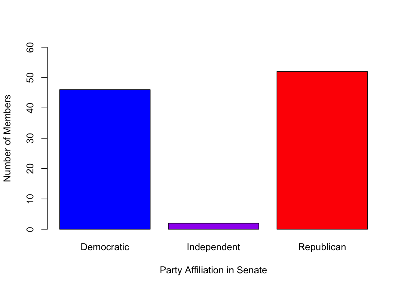
# Display the number of members by party affiliation in the senate.
table(senate$Party)
##
##  Democratic Independent  Republican
##          46           2          52
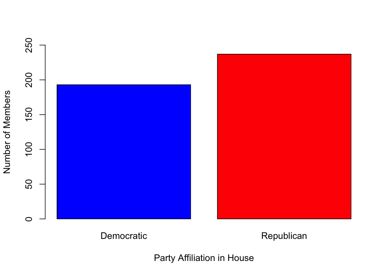
# Display the number of members by party affiliation in the house.
table(house$Party)
##
## Democratic Republican
##        193        237
# Display barplot of number of members by party affiliation in the senate.
barplot(table(senate$Party), col = c("blue", "purple", "red"), ylim = c(0, 60),
       xlab = "Party Affiliation in Senate", ylab = "Number of Members")
# Display barplot of number of members by party affiliation in the house.
barplot(table(house$Party), col = c("blue", "red"), ylim = c(0, 250),
       xlab = "Party Affiliation in House", ylab = "Number of Members")
# Display longest serving member in the senate.
senate$Name[max(senate$Years_in_office)]
## [1] Joe Manchin III
## 100 Levels: Al Franken Amy Klobuchar Angus King Ben Cardin ... Tom Udall
# Display longest serving member in the house.
house$Name[max(house$Years_in_office)]
## [1] Brendan Boyle
## 430 Levels: Adam Kinzinger Adam Schiff Adam Smith ... Zoe Lofgren
# Display table of term ending dates for "senate".
table(senate$Term_ends)
##
## January 3, 2019 January 3, 2021 January 3, 2023
##              34              32              34
# Use suggested gsub function to take values of house$District and isolate state; store in "State" vector.
State <- gsub("^(.+),.*" , "\\1" , house$District)

# Add the State vector as a column to the "house" data frame.
house$State <- State

# Display first few rows of "house" table with new "State" column.
head(house)
##                Name Years_in_office      Party    District       State
## 1    Adam Kinzinger               6 Republican District 16 District 16
## 2       Adam Schiff              16 Democratic District 28 District 28
## 3        Adam Smith              20 Democratic  District 9  District 9
## 4      Adrian Smith              10 Republican  District 3  District 3
## 5 Adriano Espaillat               0 Democratic District 13 District 13
## 6          Al Green              12 Democratic  District 9  District 9
# Display table with number of representatives for each state.
table(house$State)
##
## At-Large District        District 1       District 10       District 11
##                 6                43                13                12
##       District 12       District 13       District 14       District 15
##                11                10                 9                 7
##       District 16       District 17       District 18       District 19
##                 7                 6                 6                 4
##        District 2       District 20       District 21       District 22
##                43                 4                 4                 4
##       District 23       District 24       District 25       District 26
##                 4                 4                 4                 4
##       District 27       District 28       District 29        District 3
##                 4                 2                 2                38
##       District 30       District 31       District 32       District 33
##                 2                 2                 2                 2
##       District 34       District 35       District 36       District 37
##                 1                 2                 2                 1
##       District 38       District 39        District 4       District 40
##                 1                 1                34                 1
##       District 41       District 42       District 43       District 44
##                 1                 1                 1                 1
##       District 45       District 46       District 47       District 48
##                 1                 1                 1                 1
##       District 49        District 5       District 50       District 51
##                 1                28                 1                 1
##       District 52       District 53        District 6        District 7
##                 1                 1                25                24
##        District 8        District 9
##                21                17
# Display state with highest number of representatives.
table(house$State)[which(table(house$State) == max(table(house$State)))]
##
## District 1 District 2
##         43         43
# Display state(s) with lowest number of representatives.
table(house$State)[which(table(house$State) == min(table(house$State)))]
##
## District 34 District 37 District 38 District 39 District 40 District 41
##           1           1           1           1           1           1
## District 42 District 43 District 44 District 45 District 46 District 47
##           1           1           1           1           1           1
## District 48 District 49 District 50 District 51 District 52 District 53
##           1           1           1           1           1           1
References